How to Use a Weighted Average IF Formula in Excel

You can use the following syntax in Excel to apply a weighted average IF formula:

=SUMPRODUCT(--(A2:A7="A"), B2:B7, C2:C7)/SUMIF(A2:A7, "A", C2:C7)

This formula calculates the weighted average of the values in the range B2:B7, using C2:C7 as the weights, only for the cells where A2:A7 are equal to “A”.

The following example shows how to use this formula in practice.

Example: Weighted Average IF Formula in Excel

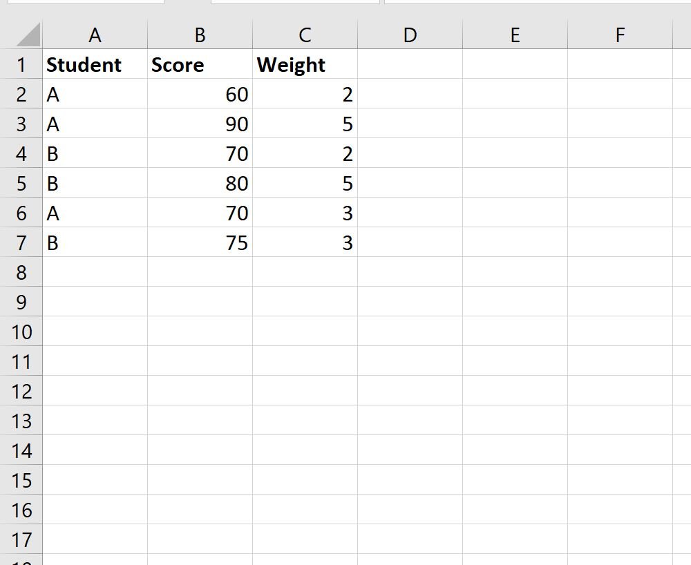
First, let’s enter the following data that shows the scores for two students (Student A and Student B) on three different exams:

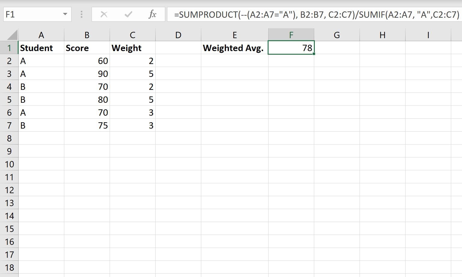
Next, we’ll use the following formula to calculate the weighted average of exam scores for student A only:

=SUMPRODUCT(--(A2:A7="A"), B2:B7, C2:C7)/SUMIF(A2:A7, "A", C2:C7)

The following screenshot shows how to use this formula in practice:

The weighted average of exam scores for student A is 78.

We can verify this is correct by manually computing the weighted average exam score for student A.

Recall that we use the following formula for weighed average:

Weighed Average = Σw_iX_i / Σw_i

where:

• w_i = the weight values
• X_i = the data values

We can plug in the values from our dataset into this formula to calculate the weighted average exam score for student A:

• Weighed Average for Student A = Σw_iX_i / Σw_i
• Weighed Average for Student A = (2*60 + 5*90 + 70*3) / (2+5+3)
• Weighed Average for Student A = 78

This matches the value that we calculated using the formula in Excel.

Additional Resources

The following tutorials explain how to perform other common tasks in Excel:

How to Calculate an Exponential Moving Average in Excel
How to Calculate a Weighted Moving Average in Excel
How to Calculate a Cumulative Average in Excel