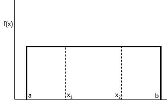
A uniform distribution is a probability distribution in which every value between an interval from a to b is equally likely to be chosen.
The probability that we will obtain a value between x1 and x2 on an interval from a to b can be found using the formula:
P(obtain value between x1 and x2) = (x2 – x1) / (b – a)
The uniform distribution has the following properties:
- The mean of the distribution is μ = (a + b) / 2
- The variance of the distribution is σ2 = (b – a)2 / 12
- The standard deviation of the distribution is σ = √σ2
Uniform Distribution in R: Syntax
The two built-in functions in R we’ll use to answer questions using the uniform distribution are:
dunif(x, min, max) – calculates the probability density function (pdf) for the uniform distribution where x is the value of a random variable, and min and max are the minimum and maximum numbers for the distribution, respectively.
punif(x, min, max) – calculates the cumulative distribution function (cdf) for the uniform distribution where x is the value of a random variable, and min and max are the minimum and maximum numbers for the distribution, respectively.
Find the full R documentation for the uniform distribution here.
Solving Problems Using the Uniform Distribution in R
Example 1: A bus shows up at a bus stop every 20 minutes. If you arrive at the bus stop, what is the probability that the bus will show up in 8 minutes or less?
Solution: Since we want to know the probability that the bus will show up in 8 minutes or less, we can simply use the punif() function since we want to know the cumulative probability that the bus will show up in 8 minute or less, given the minimum time is 0 minutes and the maximum time is 20 minutes:
punif(8, min=0, max=20)
## [1] 0.4
The probability that the bus shows up in 8 minutes or less is 0.4.
Example 2:The weight of a certain species of frog is uniformly distributed between 15 and 25 grams. If you randomly select a frog, what is the probability that the frog weighs between 17 and 19 grams?
Solution: To find the solution, we will calculate the cumulative probability of a frog weighing less than 19 pounds, then subtract the cumulative probability of a frog weighing less than 17 pounds using the following syntax:
punif(19, 15, 25) - punif(17, 15, 25)
## [1] 0.2
Thus, the probability that the frog weighs between 17 and 19 grams is 0.2.
Example 3: The length of an NBA game is uniformly distributed between 120 and 170 minutes. What is the probability that a randomly selected NBA game lasts more than 150 minutes?
Solution: To answer this question, we can use the formula 1 – (probability that the game lasts less than 150 minutes). This is given by:
1 - punif(150, 120, 170)
## [1] 0.4
The probability that a randomly selected NBA game lasts more than 150 minutes is 0.4.


