Researchers often take samples from a population and use the data from the sample to draw conclusions about the population as a whole.
One commonly used sampling method is systematic sampling, which is implemented with a simple two step process:
1. Place each member of a population in some order.
2. Choose a random starting point and select every nth member to be in the sample.
The following step-by-step example shows how to perform systematic sampling in Excel.
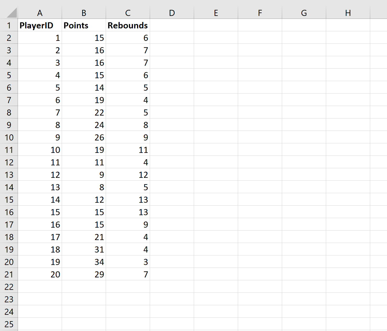
Step 1: Enter the Data
First, let’s enter the values for some dataset in Excel:
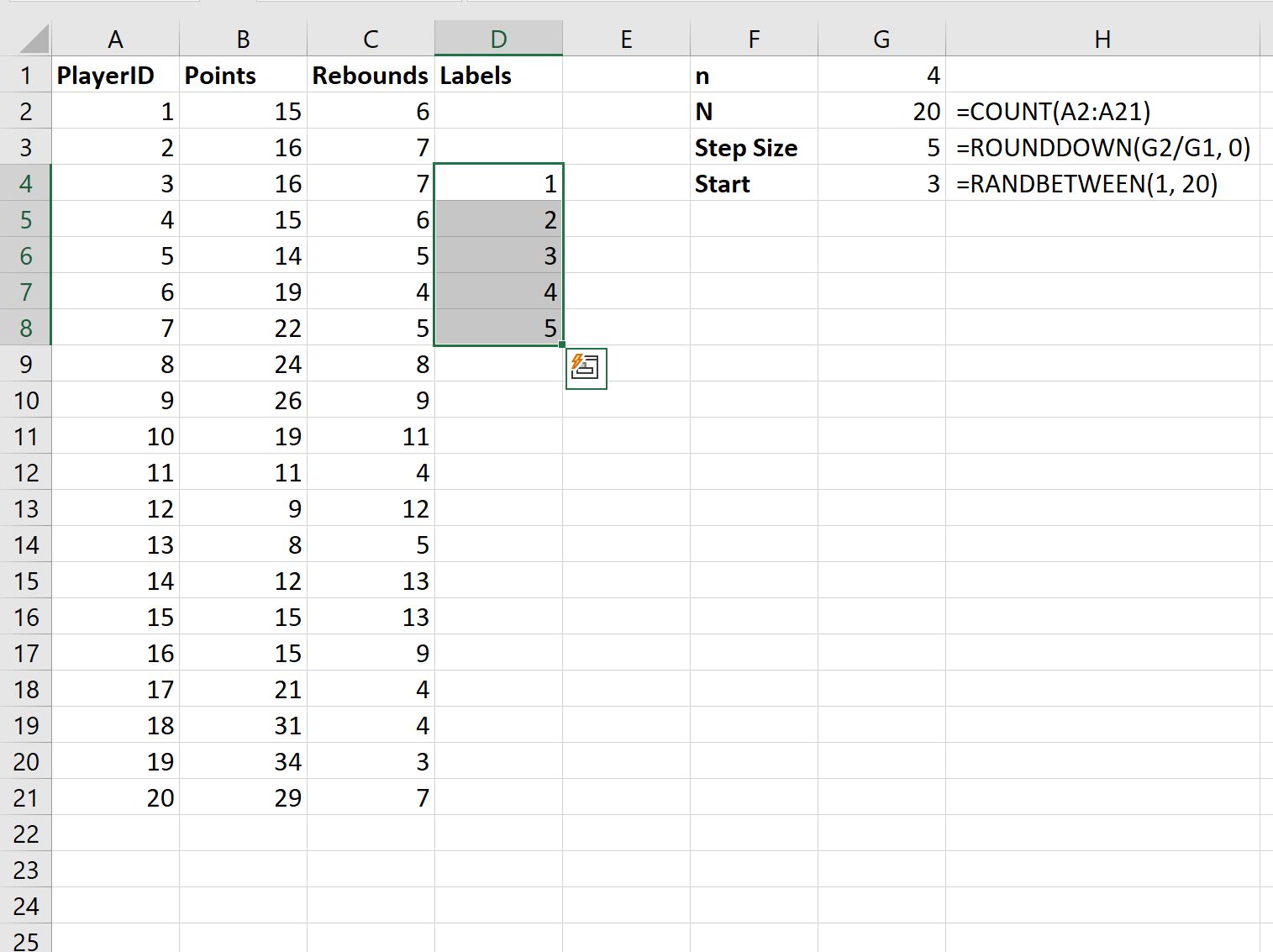
Step 2: Enter Parameter Values
Next, we need to decide how many values we’d like to randomly sample. For this example, we’ll choose a sample size of n = 4.
Next, we’ll use the following formulas to calculate the population size, step size for our systematic sampling, and random starting point:

Step 3: Label Each Data Value
Our RANDBETWEEN() function randomly chose the value 3 as the starting point in our dataset. Thus, give the data value at position 3 a label of 1 and then number down to the step size of 5:
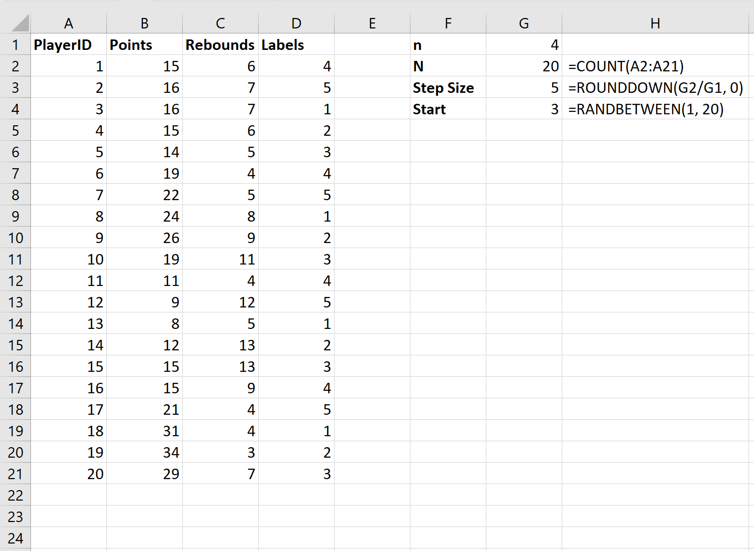
Next, type =D4 in the next available cell:

Next, copy and paste this formula down to all remaining cells in column D. Then manually fill in the values at the top of the of column D:
Step 4: Filter Values
Lastly, we need to filter the dataset to only include data values that have a label of 1.
To do so, click the Data tab along the top ribbon. Then click the Filter icon. Then click the column called Labels and filter to only include rows that have a label with value 1:

Once you do so, the data will be filtered to only include data values that have a Label of 1:

This represents our sample of size 4.
Additional Resources
Introduction to Types of Sampling Methods
How to Select a Random Sample in Excel