Often you may want to sum the cells in Google Sheets that meet one of several criteria.
You can use the following basic syntax to do so:
=SUMIFS(B2:B11, A2:A11, "value1") + SUMIFS(B2:B11, A2:A11, "value2")
This particular formula takes the sum of values in the range B2:B11 where the corresponding value in the range A2:A11 is equal to “value1” or “value2.”
The following example shows how to use this syntax in practice.
Example: Use SUMIF with OR in Google Sheets
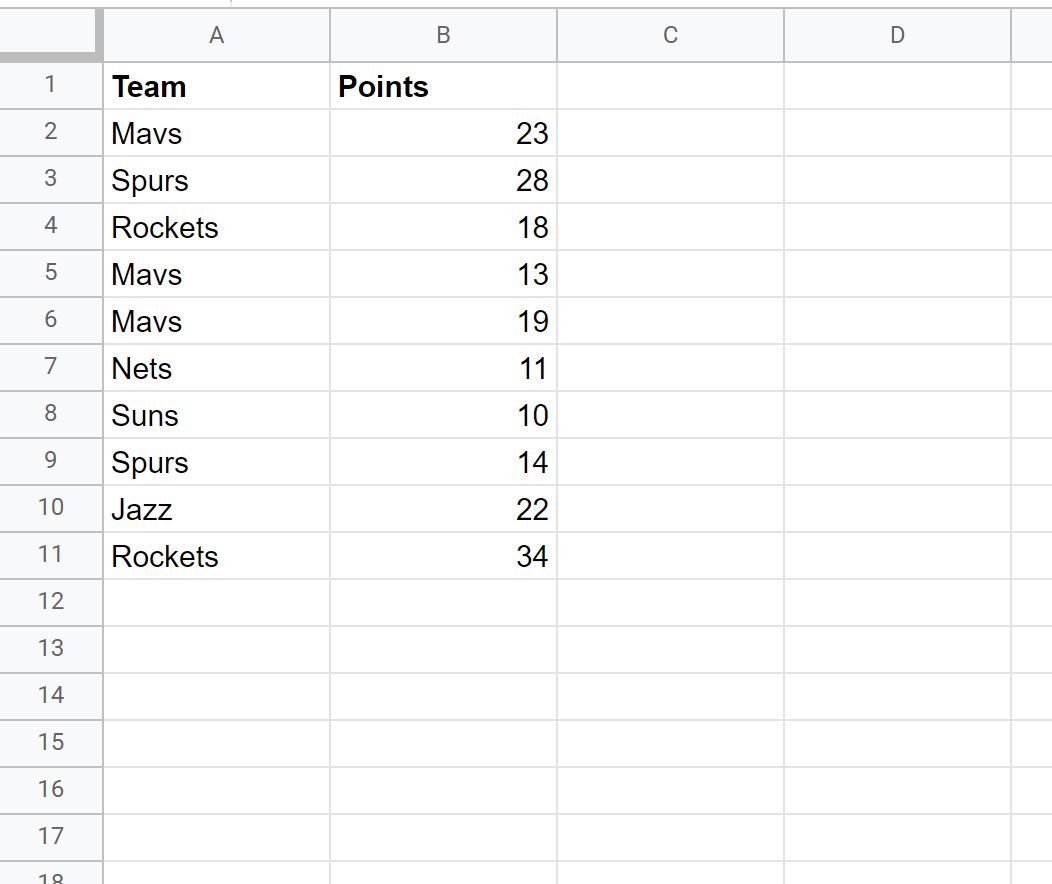
Suppose we have the following data in Google Sheets:
We can use the following formula to count the number of cells in column A that have a value of “Mavs” or “Jazz”:
=SUMIFS(B2:B11, A2:A11, "Mavs") + SUMIFS(B2:B11, A2:A11, "Jazz")
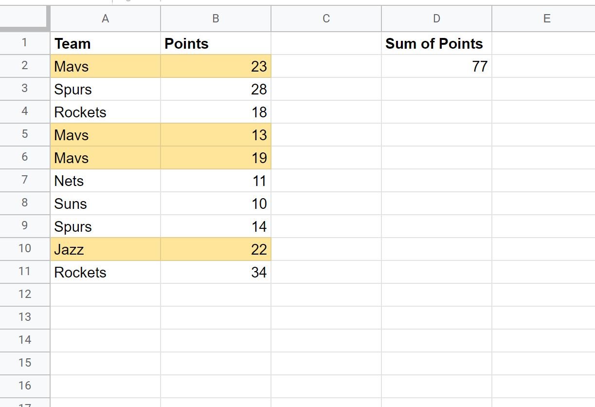
The following screenshot shows how to use this formula in practice:
We can see that the sum of values in the Points column where the corresponding value in the Team column is “Mavs” or “Jazz” is 77.
We can manually verify that this is correct by taking the sum of points for the Mavs and Jazz:
Sum of Points: 23 + 13 + 19 + 22 = 77.
Note: You can find the complete documentation for the SUMIFS function in Google Sheets here.
Additional Resources
The following tutorials explain how to perform other common SUMIF() operations in Google Sheets:
Google Sheets: How to Use SUMIFS with a Date Range
Google Sheets: How to Use SUMIF From Another Sheet
Google Sheets: How to Use SUMIF with Multiple Columns


