Simple linear regression is a method that can be used to quantify the relationship between one or more predictor variables and a response variable.
A simple linear regression model takes on the following form:
y = β0 + β1x
where:
- y: The value of the response variable
- β0: The value of the response variable when x = 0 (known as the “intercept” term)
- β1: The average increase in the response variable associated with a one unit increase in x
- x: The value of the predictor variable
A modified version of this model is known as regression through the origin, which forces y to be equal to 0 when x is equal to 0.
This type of model takes on the following form:
y = β1x
Notice that the intercept term has been completely dropped from the model.
This model is sometimes used when researchers know that the response variable must be equal to zero when the predictor variable is equal to zero.
In the real world, this type of model is used most commonly in forestry or ecology studies.
For example, researchers may use tree circumference to predict tree height. If a given tree has a circumference of zero, it must have a height of zero.
Thus, when fitting a regression model to this data it wouldn’t make sense for the intercept term to be non-zero.
The following example shows the difference between fitting an ordinary simple linear regression model compared to a model that implements regression through the origin.
Example: Regression Through the Origin
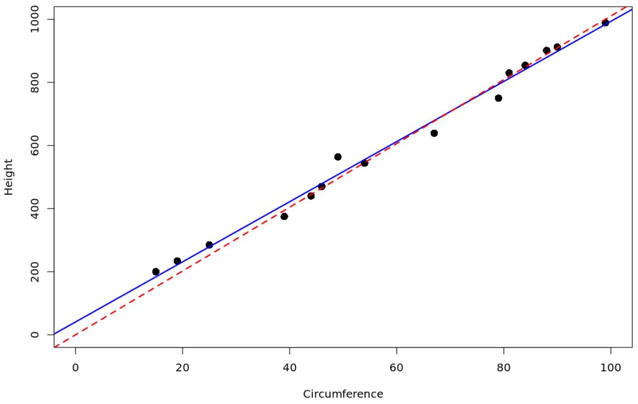
Suppose a biologist wants to fit a regression model using tree circumference to predict tree height. She goes out and collects the following measurements for a sample of 15 trees:
We can use the following code in R to fit a simple linear regression model along with a regression model that uses no intercept and plot both regression lines:
#create data frame
df frame(circ=c(15, 19, 25, 39, 44, 46, 49, 54, 67, 79, 81, 84, 88, 90, 99),
                 height=c(200, 234, 285, 375, 440, 470, 564, 544, 639, 750, 830, 854,
                          901, 912, 989))

#fit a simple linear regression model
model #fit regression through the origin
model_origin #create scatterplot
plot(df$circ, df$height, xlab='Circumference', ylab='Height',
     cex=1.5, pch=16, ylim=c(0,1000), xlim=c(0,100))

#add the fitted regression lines to the scatterplot
abline(model, col='blue', lwd=2)
abline(model_origin, lty='dashed', col='red', lwd=2)
The red dashed line represents the regression model that goes through the origin and the blue solid line represents the ordinary simple linear regression model.
We can use the following code in R to get the coefficient estimates for each model:
#display coefficients for simple linear regression model
coef(model)

(Intercept)        circ
  40.696971    9.529631

#display coefficients for regression model through the origin
coef(model_origin)

    circ
10.10574
The fitted equation for the simple linear regression model is:
Height = 40.6969 + 9.5296(Circumference)
And the fitted equation for the regression model through the origin is:
Height = 10.1057(Circumference)
Notice that the coefficient estimates for the circumference variable are slightly different.
Cautions on Using Regression Through the Origin
Before using regression through the origin, you must be absolutely sure that a value of 0 for the predictor variable implies a value of 0 for the response variable. In many scenarios, it’s almost impossible to know this for sure.
And if you’re using regression through the origin to save one degree of freedom from estimating the intercept, this rarely makes a substantial difference if your sample size is large enough.
If you do choose to use regression through the origin, be sure to state your reasoning in your final analysis or report.
Additional Resources
The following tutorials provide additional information about linear regression:
Introduction to Simple Linear Regression
Introduction to Multiple Linear Regression
How to Read and Interpret a Regression Table


