You can use the following methods to create a RANK IF formula in Google Sheets:
Method 1: RANK IF with One Criteria
=RANK(C1, FILTER(A:C, A:A="string"))
This formula finds the rank of the value in cell C1 among all values in column C where the corresponding value in column A is equal to “string.”
Method 2: RANK IF with Multiple Criteria
=RANK(C1, FILTER(A:C, A:A="string1", B:B="string2"))
This formula finds the rank of the value in cell C1 among all values in column C where the corresponding value in column A is equal to “string1” and the value in column B is equal to “string2.”
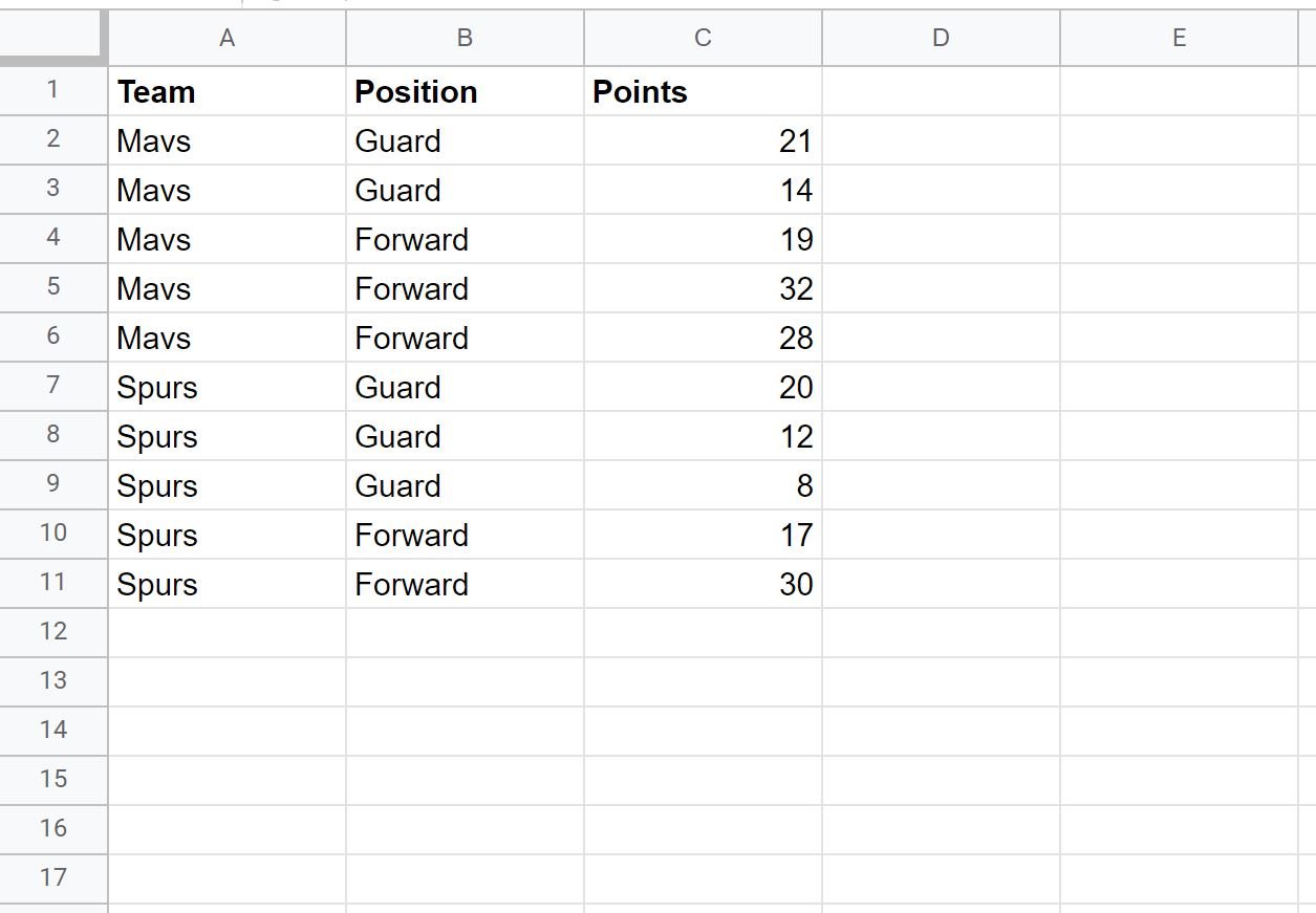
The following examples show how to use each method with the following dataset in Google Sheets:
Example 1: RANK IF with One Criteria
We can use the following formula to calculate the rank of the points values for the rows where the team is equal to “Mavs”:
=RANK(C2, FILTER(A:C, A:A="Mavs"))
The following screenshot shows how to use this syntax in practice:
Note that a rank of 1 indicates the largest value.
So, here’s how to interpret the rank values:
- The Guard on the Mavs team with 21 points has the 3rd highest points value among all players on the Mavs.
- The Guard on the Mavs team with 14 points has the 5th highest points value among all players on the Mavs.
And so on.
Note that a #N/A value was produced for each of the Spurs players since we specified in the formula that we only want to provide a ranking for players on the Mavs team.
Example 2: RANK IF with Multiple Criteria
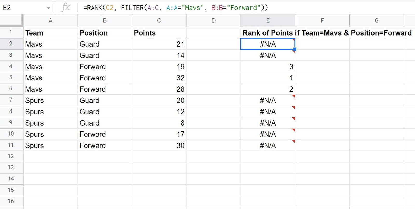
We can use the following formula to calculate the rank of the points values for the rows where the team is equal to “Mavs” and the position is equal to “Forward”:
=RANK(C2, FILTER(A:C, A:A="Mavs", B:B="Forward"))
The following screenshot shows how to use this syntax in practice:
Here’s how to interpret the rank values:
- The Forward on the Mavs team with 19 points has the 3rd highest points value among all players on the Mavs who are Forwards.
- The Forward on the Mavs team with 32 points has the 1st highest points value among all players on the Mavs who are Forwards.
And so on.
Note that a #N/A value was produced for any player who didn’t meet both criteria in our FILTER function.
Note: You can find the complete documentation for the RANK function in Google Sheets here.
Additional Resources
The following tutorials explain how to perform other common tasks in Google Sheets:
Google Sheets: How to Multiply Column by a Constant
Google Sheets: How to Multiply Column by a Percentage
Google Sheets: How to Rank Items by Multiple Columns


