You can use the following methods to create a RANK IF formula in Excel:
Method 1: RANK IF
=COUNTIFS($A$2:$A$11,A2,$B$2:$B$11,">"&B2)+1
This formula finds the rank of the value in cell B2 among all values in the range B2:B11 where the corresponding value in the range A2:A11 is equal to the value in cell A2.
Using this method, the largest value is assigned a value of 1.
Method 2: Reverse RANK IF
=COUNTIFS($A$2:$A$11,A2,$B$2:$B$11,"B2)+1
This formula finds the rank of the value in cell B2 among all values in the range B2:B11 where the corresponding value in the range A2:A11 is equal to the value in cell A2.
Using this method, the smallest value is assigned a value of 1.
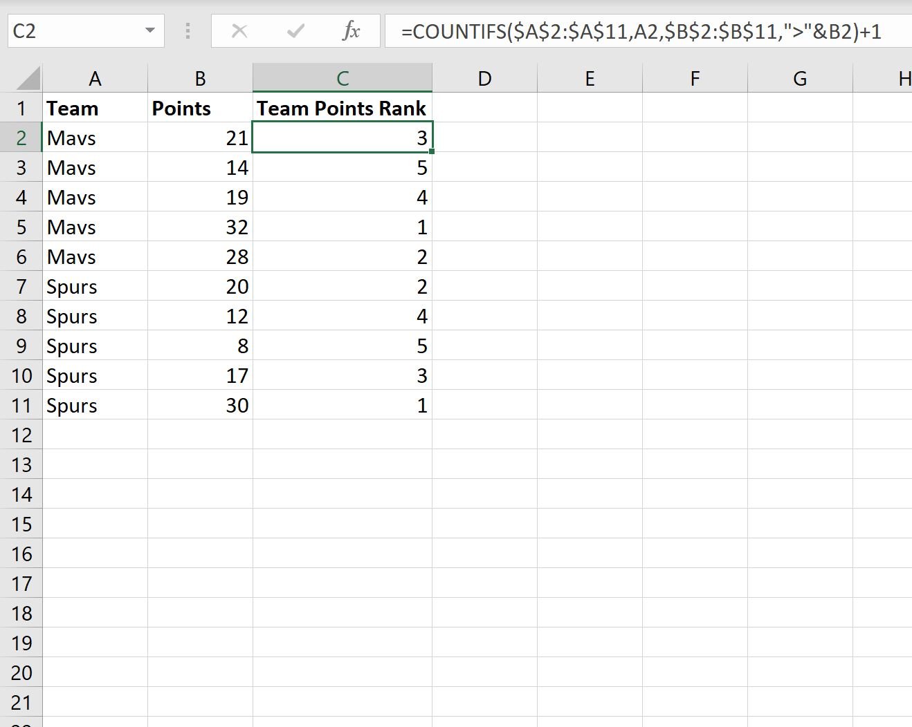
The following examples show how to use each method with the following dataset in Excel:
Example 1: RANK IF
We can type the following formula into cell C2 to calculate the rank of the points value in cell B2 among all players on the “Mavs” team:
=COUNTIFS($A$2:$A$11,A2,$B$2:$B$11,">"&B2)+1
We can then drag this formula down to each remaining cell in column C:
Here’s how to interpret the output:
- The first player scored the 3rd most points among all players on the Mavs team.
- The second player scored the 5th most points among all players on the Mavs team.
And so on.
Using this formula, the player with the highest points value on each team receives a rank of 1.
Example 2: Reverse RANK IF
We can type the following formula into cell C2 to calculate the rank of the points value in cell B2 among all players on the “Mavs” team:
=COUNTIFS($A$2:$A$11,A2,$B$2:$B$11,"B2)+1
We can then drag this formula down to each remaining cell in column C:
Here’s how to interpret the output:
- The first player scored the 3rd lowest points among all players on the Mavs team.
- The second player scored the 1st lowest points among all players on the Mavs team.
And so on.
Using this formula, the player with the lowest points value on each team receives a rank of 1.
Additional Resources
The following tutorials explain how to perform other common tasks in Excel:
How to Calculate Percentile Rank in Excel
How to Rank Values by Group in Excel
How to Rank Items by Multiple Criteria in Excel


