Linear regression is a method we can use to understand the relationship between one or more explanatory variables and a response variable.
When we perform linear regression on a dataset, we end up with a regression equation which can be used to predict the values of a response variable, given the values for the explanatory variables.
We can then measure the difference between the predicted values and the actual values to come up with the residuals for each prediction. This helps us get an idea of how well our regression model is able to predict the response values.
This tutorial explains how to obtain both the predicted values and the residuals for a regression model in Stata.
Example: How to Obtain Predicted Values and Residuals
For this example we will use the built-in Stata dataset called auto. We’ll use mpg and displacement as the explanatory variables and price as the response variable.
Use the following steps to perform linear regression and subsequently obtain the predicted values and residuals for the regression model.
Step 1: Load and view the data.
First, we’ll load the data using the following command:
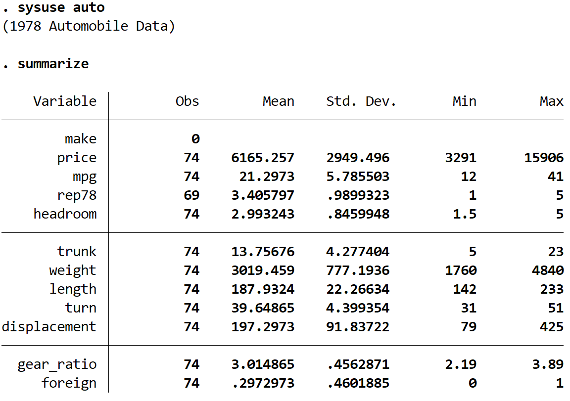
sysuse auto
Next, we’ll get a quick summary of the data using the following command:
summarize
Step 2: Fit the regression model.
Next, we’ll use the following command to fit the regression model:
regress price mpg displacement
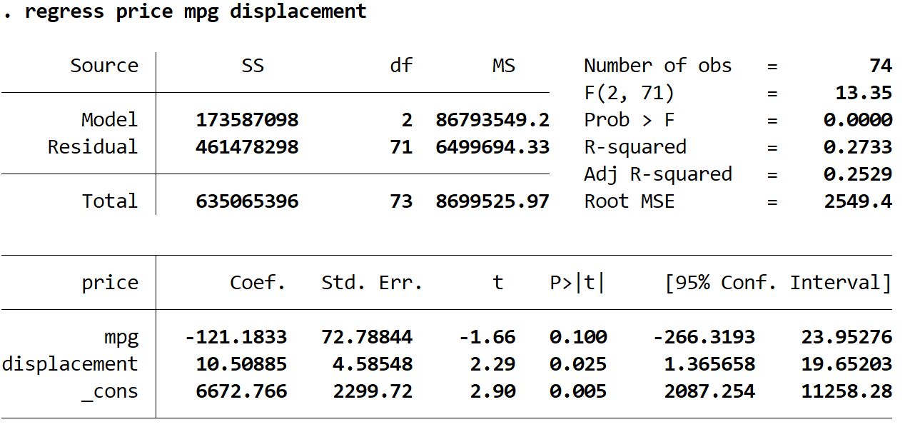
The estimated regression equation is as follows:
estimated price = 6672.766 -121.1833*(mpg) + 10.50885*(displacement)
Step 3: Obtain the predicted values.
We can obtain the predicted values by using the predict command and storing these values in a variable named whatever we’d like. In this case, we’ll use the name pred_price:
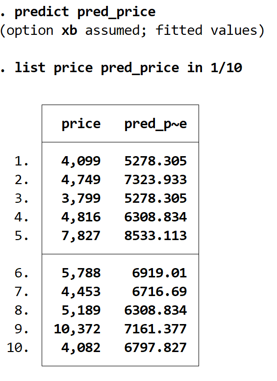
predict pred_price
We can view the actual prices and the predicted prices side-by-side using the list command. There are 74 total predicted values, but we’ll view just the first 10 by using the in 1/10 command:
list price pred_price in 1/10
Step 4: Obtain the residuals.
We can obtain the residuals of each prediction by using the residuals command and storing these values in a variable named whatever we’d like. In this case, we’ll use the name resid_price:
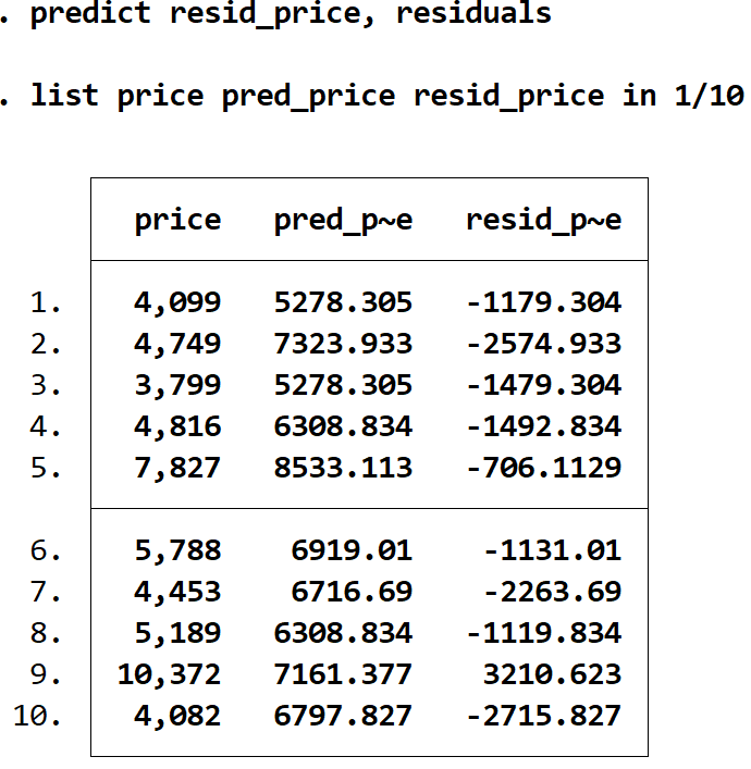
predict resid_price, residuals
We can view the actual price, the predicted price, and the residuals all side-by-side using the list command again:
list price pred_price resid_price in 1/10
Step 5: Create a predicted values vs. residuals plot.
Lastly, we can created a scatterplot to visualize the relationship between the predicted values and the residuals:
scatter resid_price pred_price
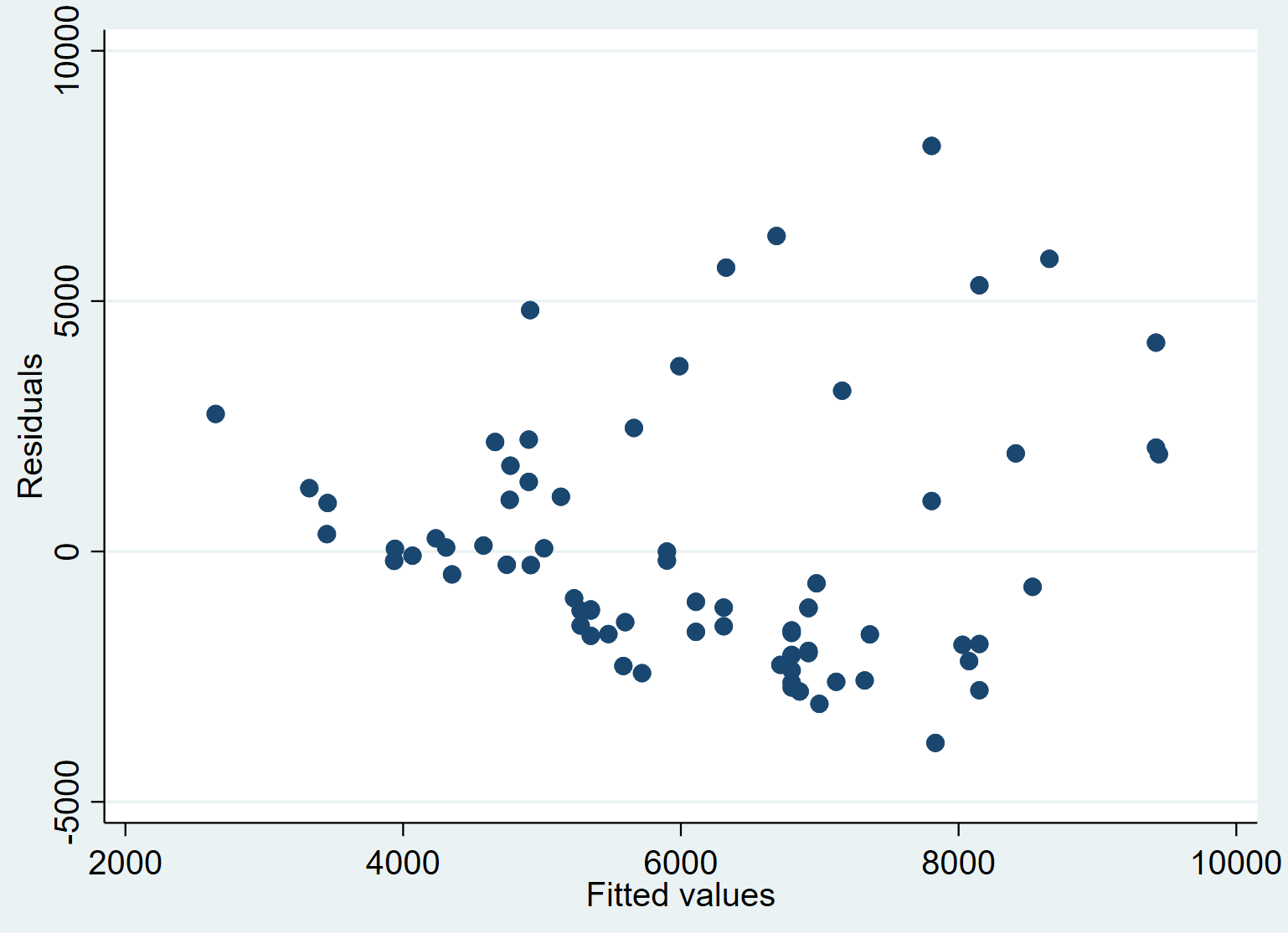
We can see that, on average, the residuals tend to grow larger as the fitted values grow larger. This could be a sign of heteroscedasticity – when the spread of the residuals is not constant at every response level.
We could formally test for heteroscedasticity using the Breusch-Pagan Test and we could address this problem using robust standard errors.