How to Perform Power Regression in R (Step-by-Step)

Power regression is a type of non-linear regression that takes on the following form:

y = ax^b

where:

• y: The response variable
• x: The predictor variable
• a, b: The regression coefficients that describe the relationship between x and y

This type of regression is used to model situations where the response variable is equal to the predictor variable raised to a power.

The following step-by-step example shows how to perform power regression for a given dataset in R.

Step 1: Create the Data

First, let’s create some fake data for two variables: x and y.

#create data
x=1:20
y=c(1, 8, 5, 7, 6, 20, 15, 19, 23, 37, 33, 38, 49, 50, 56, 52, 70, 89, 97, 115) 

Step 2: Visualize the Data

Next, let’s create a scatterplot to visualize the relationship between x and y:

#create scatterplot
plot(x, y)

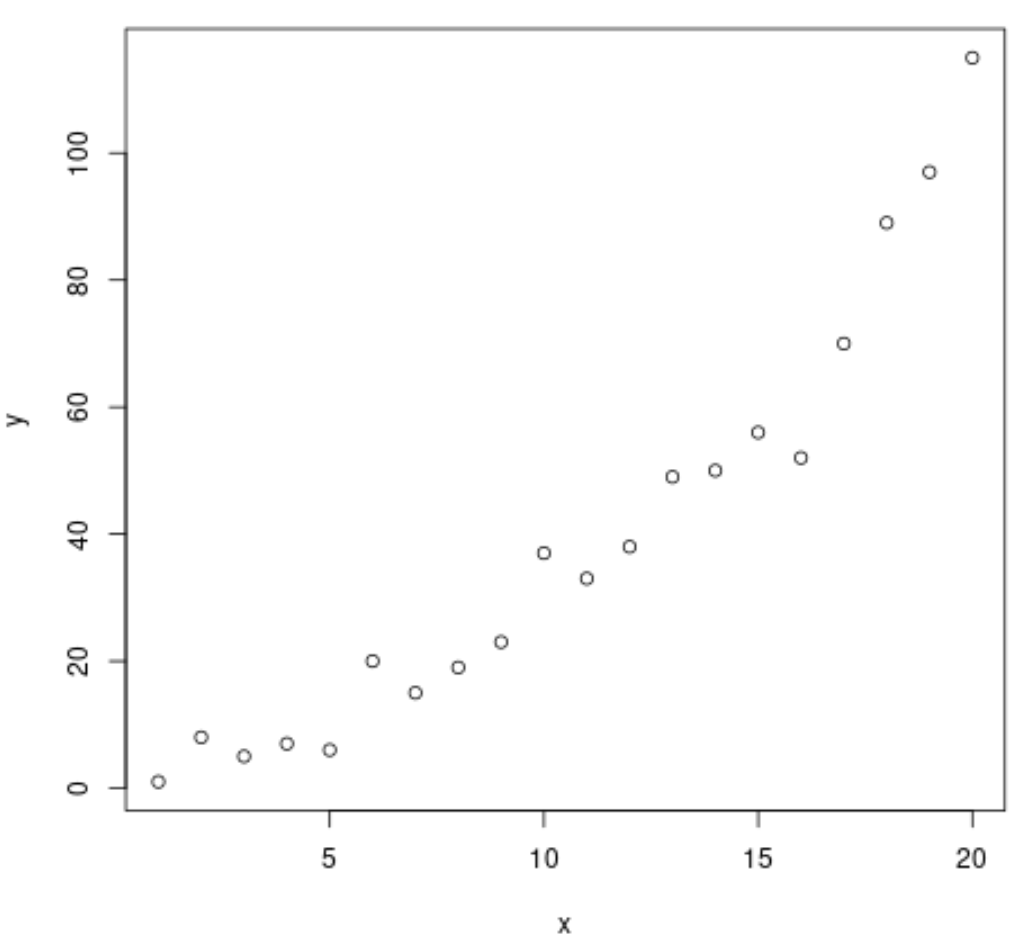
From the plot we can see that there exists a clear power relationship between the two variables. Thus, it seems like a good idea to fit a power regression equation to the data instead of a linear regression model.

Step 3: Fit the Power Regression Model

Next, we’ll use the lm() function to fit a regression model to the data, specifying that R should use the log of the response variable and the log of the predictor variable when fitting the model:

#fit the model
model #view the output of the model
summary(model)

Call:
lm(formula = log(y) ~ log(x))

Residuals:
     Min       1Q   Median       3Q      Max 
-0.67014 -0.17190 -0.05341  0.16343  0.93186 

Coefficients:
            Estimate Std. Error t value Pr(>|t|)    
(Intercept)  0.15333    0.20332   0.754    0.461    
log(x)       1.43439    0.08996  15.945 4.62e-12 ***
---
Signif. codes:  0 ‘***’ 0.001 ‘**’ 0.01 ‘*’ 0.05 ‘.’ 0.1 ‘ ’ 1

Residual standard error: 0.3187 on 18 degrees of freedom
Multiple R-squared:  0.9339,	Adjusted R-squared:  0.9302 
F-statistic: 254.2 on 1 and 18 DF,  p-value: 4.619e-12

The overall F-value of the model is 252.1 and the corresponding p-value is extremely small (4.619e-12), which indicates that the model as a whole is useful.

Using the coefficients from the output table, we can see that the fitted power regression equation is:

ln(y) = 0.15333 + 1.43439ln(x)

Applying e to both sides, we can rewrite the equation as:

• y = e ^{0.15333 + 1.43439ln(x)}
• y = 1.1657x^1.43439

We can use this equation to predict the response variable, y, based on the value of the predictor variable, x.

For example, if x = 12, then we would predict that y would be 41.167:

y = 1.1657(12)^1.43439 = 41.167

Bonus: Feel free to use this online Power Regression Calculator to automatically compute the power regression equation for a given predictor and response variable.

Additional Resources

How to Perform Multiple Linear Regression in R
How to Perform Exponential Regression in R
How to Perform Logarithmic Regression in R