A population pyramid is a graph that shows the age and gender distribution of a given population. It’s useful for understanding the composition of a population and the trend in population growth.
This tutorial explains how to create the following population pyramid in Excel:
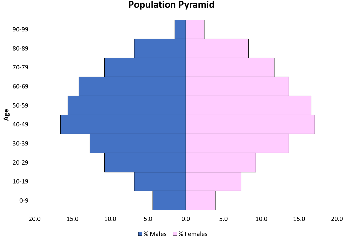
Example: Population Pyramid in Excel
Use the following steps to create a population pyramid in Excel.
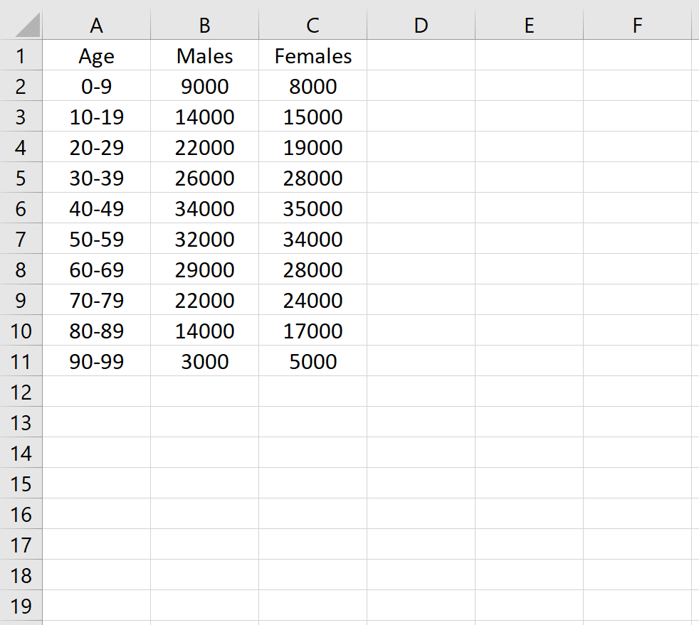
Step 1: Input the data.
First, input the population counts (by age bracket) for males and females in separate columns:
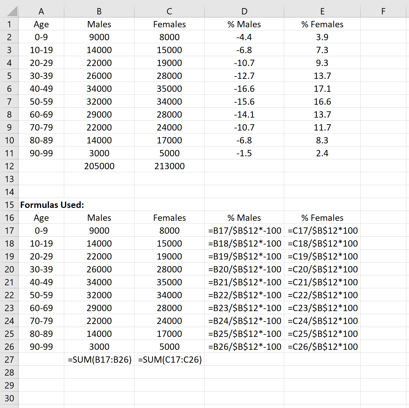
Step 2: Calculate the percentages.
Next, use the following formulas to calculate the percentages for both males and females:
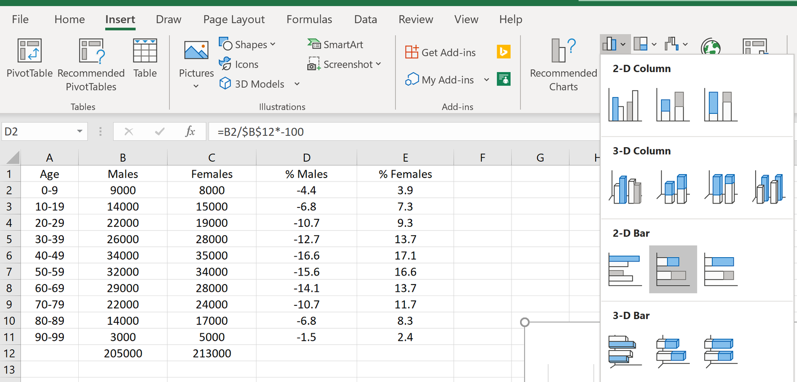
Step 3: Insert a 2-D Stacked Bar Chart.
Next, highlight cells D2:E:11. In the Charts group within the Insert tab, click on the option that says 2-D stacked bar chart:
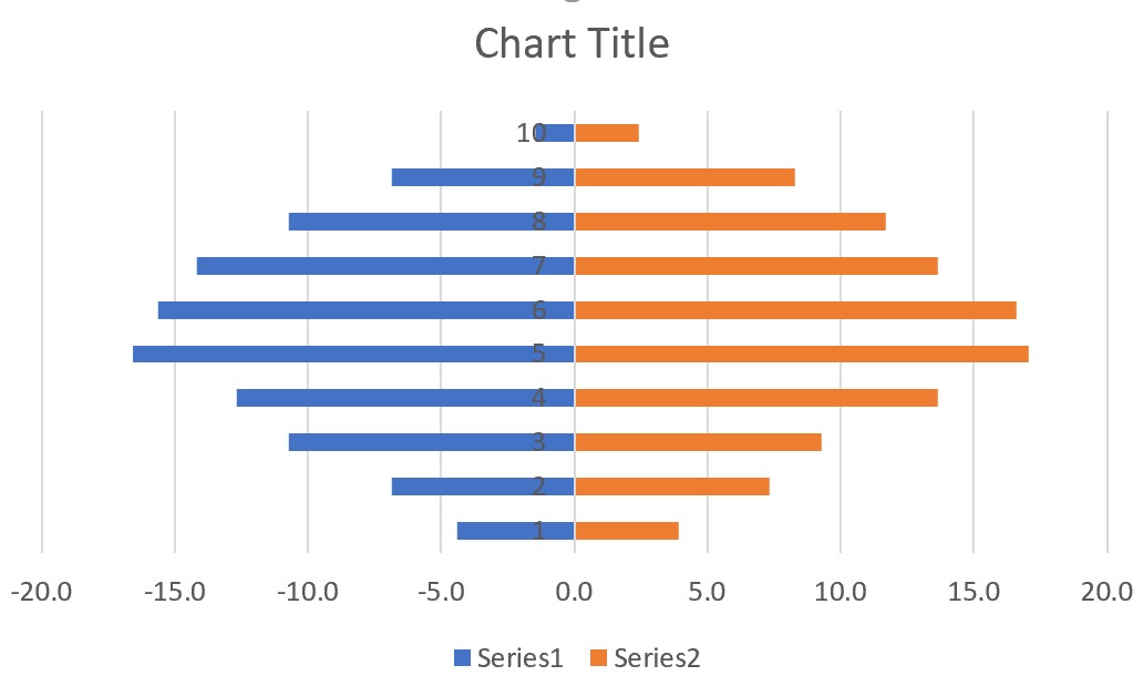
The following chart will automatically appear:
Step 4: Modify the appearance of the population pyramid.
Lastly, we will modify the appearance of the population pyramid to make it look better.
Remove the gap width.
- Right click any bar on the chart. Then click Format Data Series…
- Change Gap Width to 0%.

Add a black border to each bar.
- Click the paint bucket icon.
- Click Border. Then click Solid line.
- Change the Color to black.

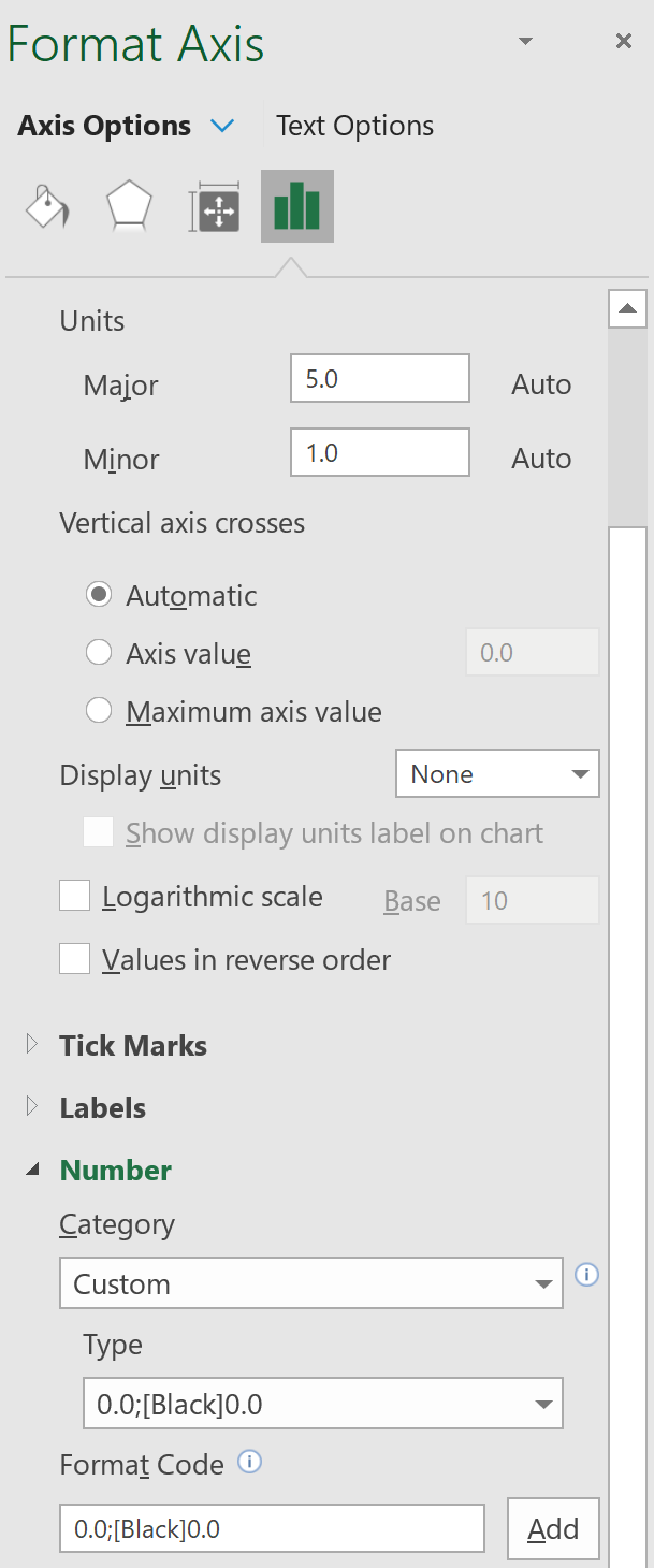
Display the x-axis labels as positive numbers.
- Right click on the x-axis. Then click Format Axis…
- Click Number.
- Under Format Code, type 0.0;[Black]0.0 and click Add.
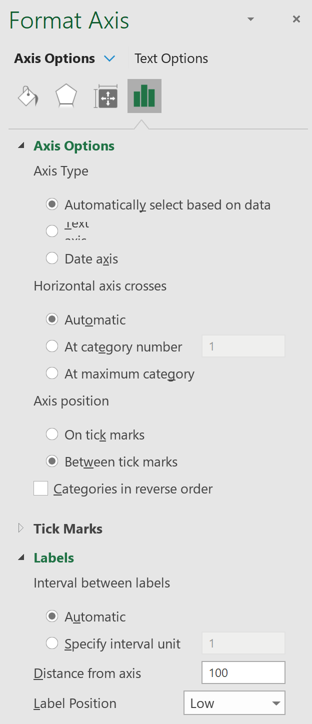
Move the vertical axis to the left-hand side of the chart.
- Right click on the y-axis. Then click Format Axis…
- Click Labels. Set Label Position to Low.
Change the title of the graph and the colors as needed. Also click on any of the vertical grid lines and click delete.
The final result should look like this: