How to Perform Polynomial Regression in Python

Regression analysis is used to quantify the relationship between one or more explanatory variables and a response variable.

The most common type of regression analysis is simple linear regression, which is used when a predictor variable and a response variable have a linear relationship.

However, sometimes the relationship between a predictor variable and a response variable is nonlinear.

For example, the true relationship may be quadratic:

Or it may be cubic:

In these cases it makes sense to use polynomial regression, which can account for the nonlinear relationship between the variables.

This tutorial explains how to perform polynomial regression in Python.

Example: Polynomial Regression in Python

Suppose we have the following predictor variable (x) and response variable (y) in Python:

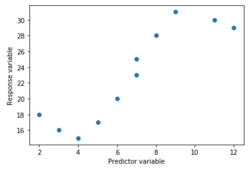
x = [2, 3, 4, 5, 6, 7, 7, 8, 9, 11, 12]
y = [18, 16, 15, 17, 20, 23, 25, 28, 31, 30, 29]

If we create a simple scatterplot of this data, we can see that the relationship between x and y is clearly not linear:

import matplotlib.pyplot as plt

#create scatterplot 
plt.scatter(x, y)

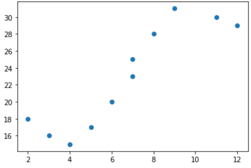
Thus, it wouldn’t make sense to fit a linear regression model to this data. Instead, we can attempt to fit a polynomial regression model with a degree of 3 using the numpy.polyfit() function:

import numpy as np

#polynomial fit with degree = 3
model = np.poly1d(np.polyfit(x, y, 3))

#add fitted polynomial line to scatterplot
polyline = np.linspace(1, 12, 50)
plt.scatter(x, y)
plt.plot(polyline, model(polyline))
plt.show()

We can obtain the fitted polynomial regression equation by printing the model coefficients:

print(model)

poly1d([ -0.10889554,   2.25592957, -11.83877127,  33.62640038])

The fitted polynomial regression equation is:

y = -0.109x³ + 2.256x² – 11.839x + 33.626

This equation can be used to find the expected value for the response variable based on a given value for the explanatory variable. For example, suppose x = 4. The expected value for the response variable, y, would be:

y = -0.109(4)³ + 2.256(4)² – 11.839(4) + 33.626= 15.39.

We can also write a short function to obtain the R-squared of the model, which is the proportion of the variance in the response variable that can be explained by the predictor variables.

#define function to calculate r-squared
def polyfit(x, y, degree):
    results = {}
    coeffs = numpy.polyfit(x, y, degree)
    p = numpy.poly1d(coeffs)
    #calculate r-squared
    yhat = p(x)
    ybar = numpy.sum(y)/len(y)
    ssreg = numpy.sum((yhat-ybar)**2)
    sstot = numpy.sum((y - ybar)**2)
    results['r_squared'] = ssreg / sstot

    return results

#find r-squared of polynomial model with degree = 3
polyfit(x, y, 3)

{'r_squared': 0.9841113454245183}

In this example, the R-squared of the model is 0.9841. This means that 98.41% of the variation in the response variable can be explained by the predictor variables.