In machine learning, a decision tree is a type of model that uses a set of predictor variables to build a decision tree that predicts the value of a response variable.
The easiest way to plot a decision tree in R is to use the prp() function from the rpart.plot package.
The following example shows how to use this function in practice.
Example: Plotting a Decision Tree in R
For this example, we’ll use the Hitters dataset from the ISLR package, which contains various information about 263 professional baseball players.
We will use this dataset to build a regression tree that uses home runs and years played to predict the salary of a given player.
The following code shows how to fit this regression tree and how to use the prp() function to plot the tree:
library(ISLR)
library(rpart)
library(rpart.plot)

#build the initial decision tree
tree control(cp=.0001))

#identify best cp value to use
best min(tree$cptable[,"xerror"]),"CP"]

#produce a pruned tree based on the best cp value
pruned_tree prune(tree, cp=best)

#plot the pruned tree
prp(pruned_tree)

Note that we can also customize the appearance of the decision tree by using the faclen, extra, roundint, and digits arguments within the prp() function:
#plot decision tree using custom arguments
prp(pruned_tree,
    faclen=0, #use full names for factor labels
    extra=1, #display number of observations for each terminal node
    roundint=F, #don't round to integers in output
    digits=5) #display 5 decimal places in output
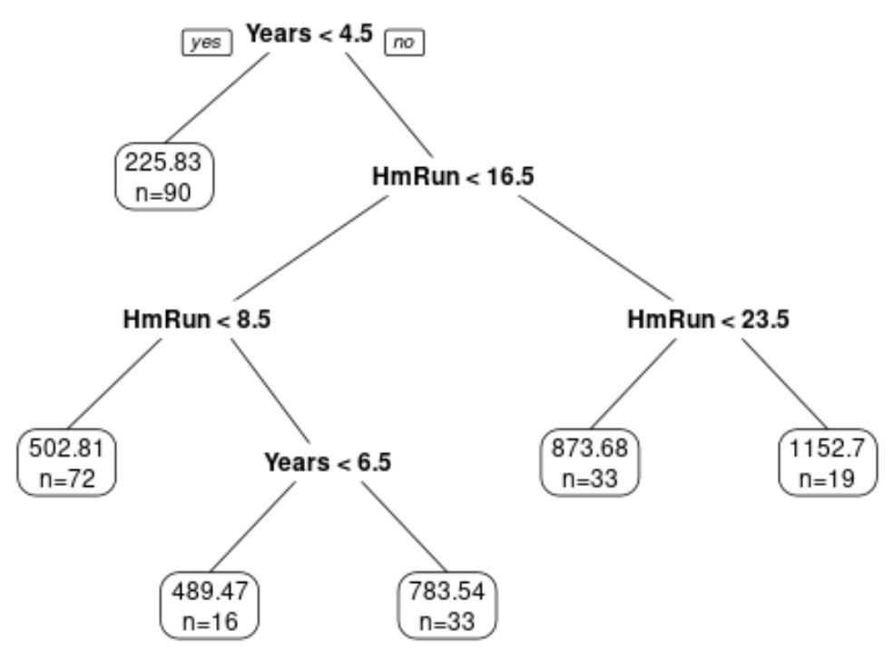
We can see that the tree has six terminal nodes.
Each terminal node shows the predicted salary of players in that node along with the number of observations from the original dataset that belong to that note.
For example, we can see that in the original dataset there were 90 players with less than 4.5 years of experience and their average salary was $225.83k.

We can also use the tree to predict a given player’s salary based on their years of experience and average home runs.
For example, a player who has 7 years of experience and 4 average home runs has a predicted salary of $502.81k.

This is one advantage of using a decision tree: We can easily visualize and interpret the results.
Additional Resources
The following tutorials provide additional information about decision trees:
An Introduction to Classification and Regression Trees
Decision Tree vs. Random Forests: What’s the Difference?
How to Fit Classification and Regression Trees in R