Understanding the Null Hypothesis for Linear Regression

Linear regression is a technique we can use to understand the relationship between one or more predictor variables and a response variable.

If we only have one predictor variable and one response variable, we can use simple linear regression, which uses the following formula to estimate the relationship between the variables:

ŷ = β₀ + β₁x

where:

• ŷ: The estimated response value.
• β₀: The average value of y when x is zero.
• β₁: The average change in y associated with a one unit increase in x.
• x: The value of the predictor variable.

Simple linear regression uses the following null and alternative hypotheses:

• H₀: β₁ = 0
• H_A: β₁ ≠ 0

The null hypothesis states that the coefficient β₁ is equal to zero. In other words, there is no statistically significant relationship between the predictor variable, x, and the response variable, y.

The alternative hypothesis states that β₁ is not equal to zero. In other words, there is a statistically significant relationship between x and y.

If we have multiple predictor variables and one response variable, we can use multiple linear regression, which uses the following formula to estimate the relationship between the variables:

ŷ = β₀ + β₁x₁ + β₂x₂ + … + β_kx_k

where:

• ŷ: The estimated response value.
• β₀: The average value of y when all predictor variables are equal to zero.
• β_i: The average change in y associated with a one unit increase in x_i.
• x_i: The value of the predictor variable x_i.

Multiple linear regression uses the following null and alternative hypotheses:

• H₀: β₁ = β₂ = … = β_k = 0
• H_A: β₁ = β₂ = … = β_k ≠ 0

The null hypothesis states that all coefficients in the model are equal to zero. In other words, none of the predictor variables have a statistically significant relationship with the response variable, y.

The alternative hypothesis states that not every coefficient is simultaneously equal to zero.

The following examples show how to decide to reject or fail to reject the null hypothesis in both simple linear regression and multiple linear regression models.

Example 1: Simple Linear Regression

Suppose a professor would like to use the number of hours studied to predict the exam score that students will receive in his class. He collects data for 20 students and fits a simple linear regression model.

The following screenshot shows the output of the regression model:

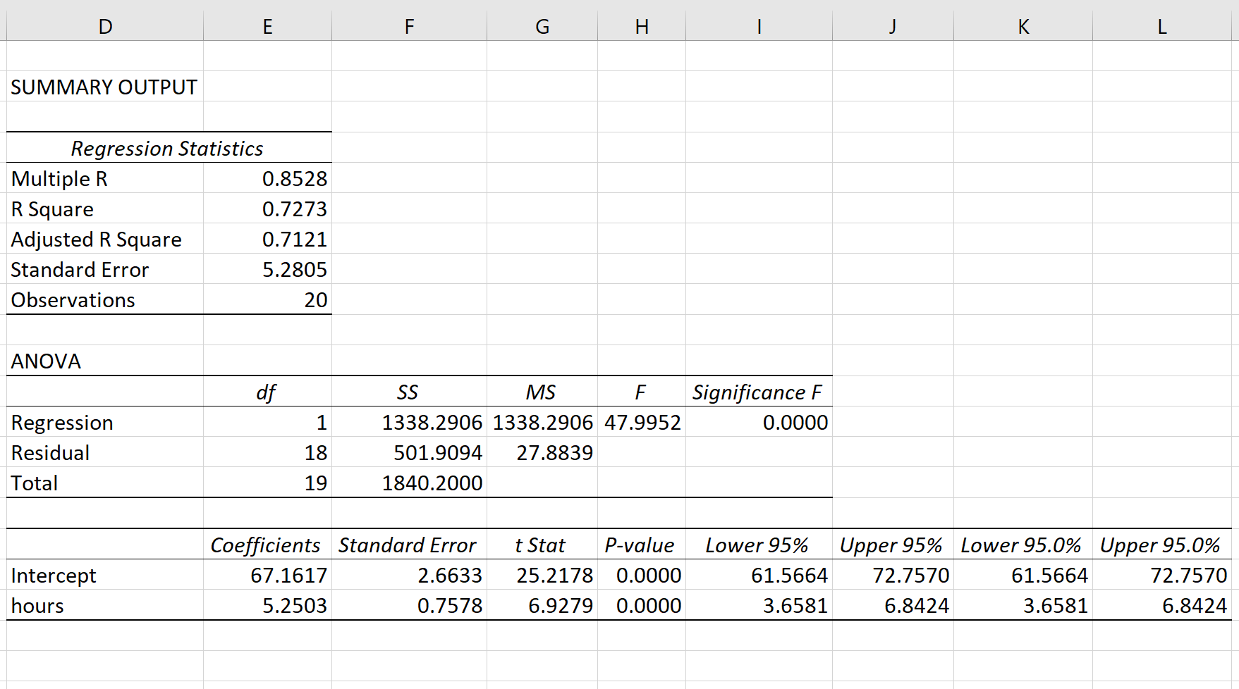
The fitted simple linear regression model is:

Exam Score = 67.1617 + 5.2503*(hours studied)

To determine if there is a statistically significant relationship between hours studied and exam score, we need to analyze the overall F value of the model and the corresponding p-value:

• Overall F-Value: 47.9952
• P-value: 0.000

Since this p-value is less than .05, we can reject the null hypothesis. In other words, there is a statistically significant relationship between hours studied and exam score received.

Example 2: Multiple Linear Regression

Suppose a professor would like to use the number of hours studied and the number of prep exams taken to predict the exam score that students will receive in his class. He collects data for 20 students and fits a multiple linear regression model.

The following screenshot shows the output of the regression model:

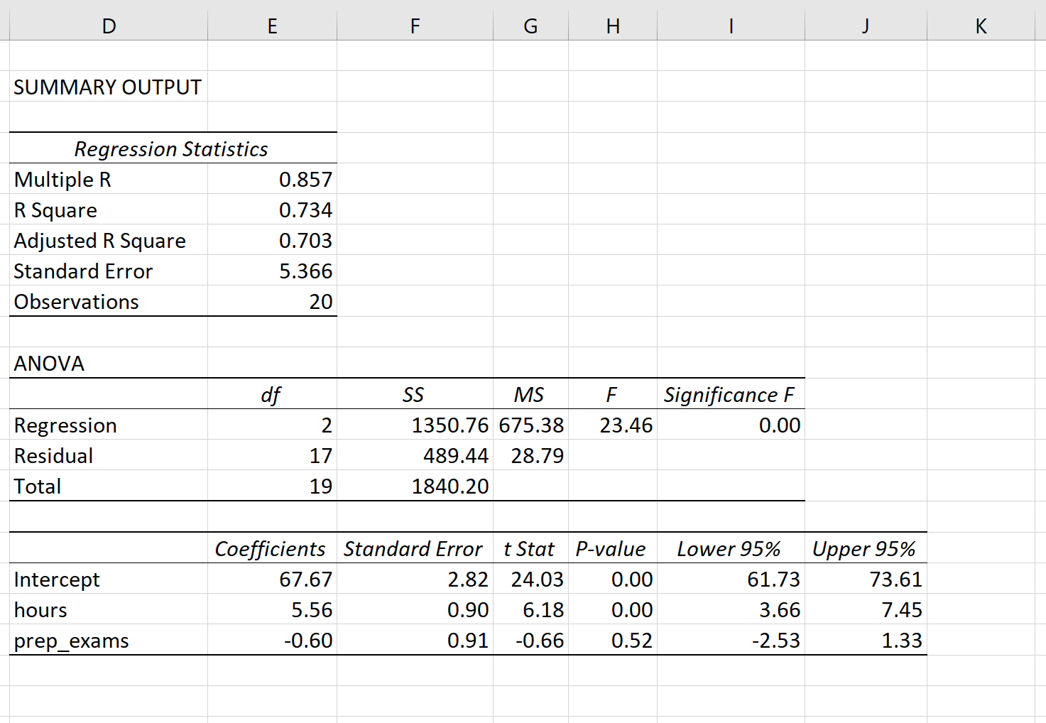
The fitted multiple linear regression model is:

Exam Score = 67.67 + 5.56*(hours studied) – 0.60*(prep exams taken)

To determine if there is a jointly statistically significant relationship between the two predictor variables and the response variable, we need to analyze the overall F value of the model and the corresponding p-value:

• Overall F-Value: 23.46
• P-value: 0.00

Since this p-value is less than .05, we can reject the null hypothesis. In other words, hours studied and prep exams taken have a jointly statistically significant relationship with exam score.

Note: Although the p-value for prep exams taken (p = 0.52) is not significant, prep exams combined with hours studied has a significant relationship with exam score.

Additional Resources

Understanding the F-Test of Overall Significance in Regression
How to Read and Interpret a Regression Table
How to Report Regression Results
How to Perform Simple Linear Regression in Excel
How to Perform Multiple Linear Regression in Excel