Logistic Regression is a method that we use to fit a regression model when the response variable is binary. Here are some examples of when we may use logistic regression:
- We want to know how exercise, diet, and weight impact the probability of having a heart attack. The response variable is heart attack and it has two potential outcomes: a heart attack occurs or does not occur.
- We want to know how GPA, ACT score, and number of AP classes taken impact the probability of getting accepted into a particular university. The response variable is acceptance and it has two potential outcomes: accepted or not accepted.
- We want to know whether word count and email title impact the probability that an email is spam. The response variable is spam and it has two potential outcomes: spam or not spam.
This tutorial explains how to perform logistic regression in Stata.
Example: Logistic Regression in Stata
Suppose we are interested in understanding whether a mother’s age and her smoking habits affect the probability of having a baby with a low birthweight.
To explore this, we can perform logistic regression using age and smoking (either yes or no) as explanatory variables and low birthweight (either yes or no) as a response variable. Since the response variable is binary – there are only two possible outcomes – it is appropriate to use logistic regression.
Perform the following steps in Stata to conduct a logistic regression using the dataset called lbw, which contains data on 189 different mothers.
Step 1: Load the data.
Load the data by typing the following into the Command box:
use https://www.stata-press.com/data/r13/lbw
Step 2: Get a summary of the data.
Gain a quick understanding of the data you’re working with by typing the following into the Command box:
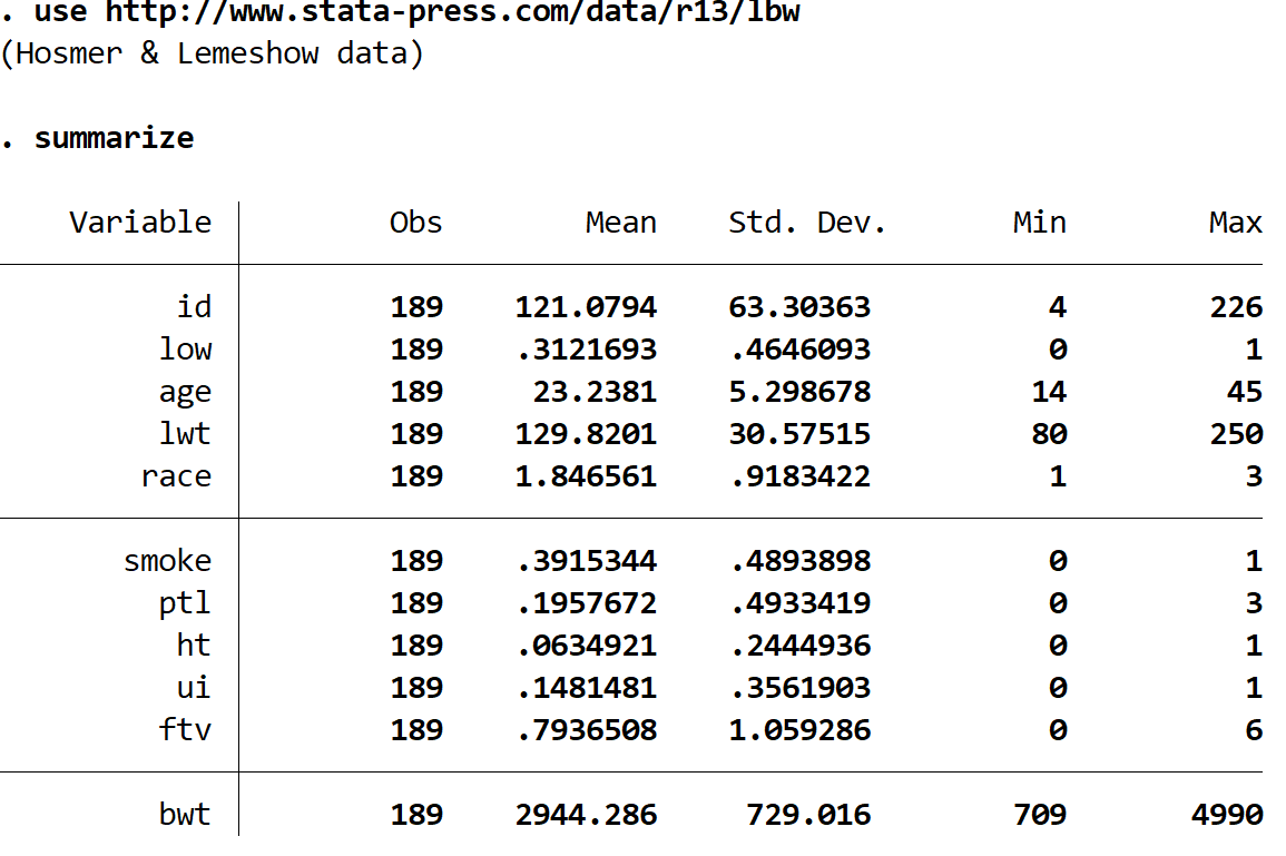
summarize
We can see that there are 11 different variables in the dataset, but the only three that we care about are the following:
- low – whether or not the baby had a low birthweight. 1 = yes, 0 = no.
- age – age of the mother.
- smoke – whether or not the mother smoked during pregnancy. 1 = yes, 0 = no.
Step 3: Perform logistic regression.
Type the following into the Command box to perform logistic regression using age and smoke as explanatory variables and low as the response variable.
logit low age smoke
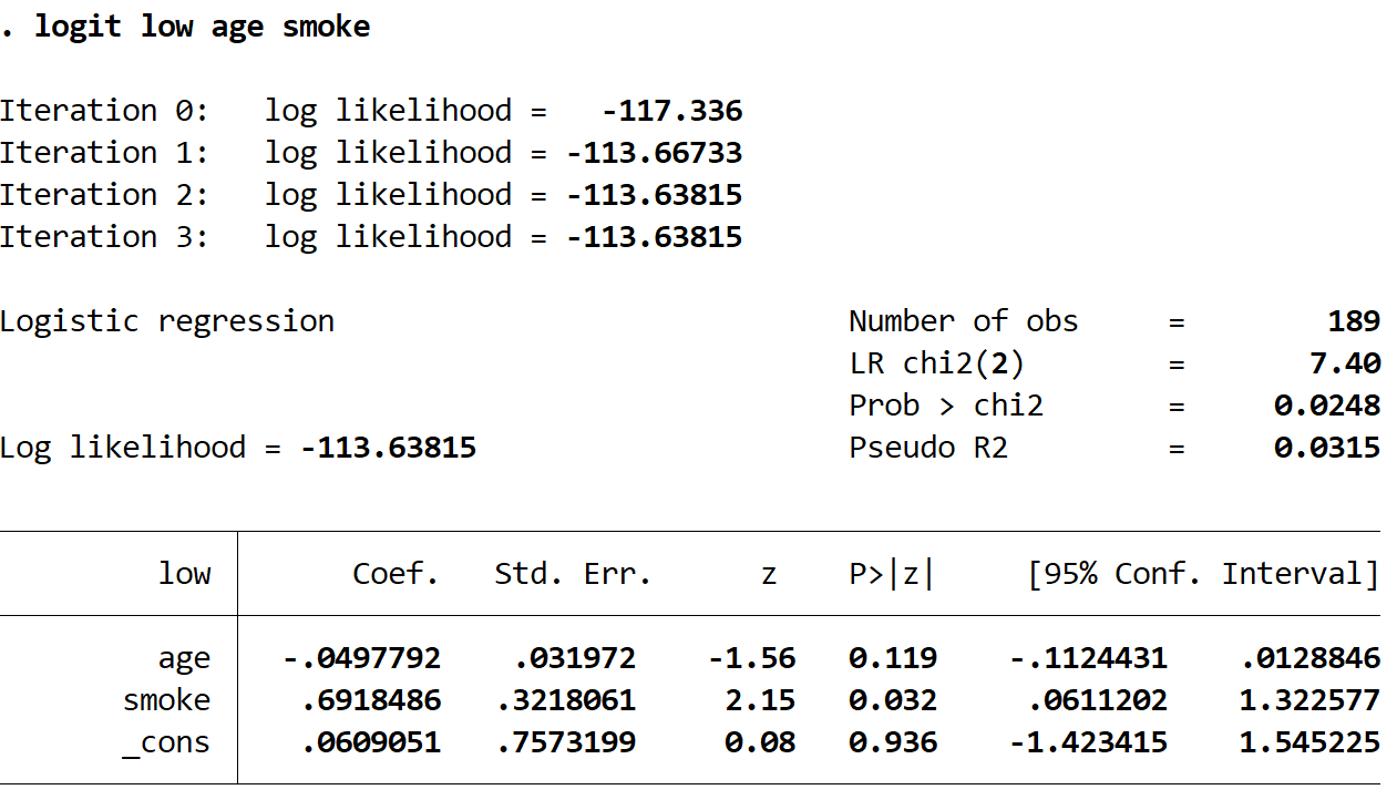
Here is how to interpret the most interesting numbers in the output:
Coef (age): -.0497792. Holding smoke constant, each one year increase in age is associated with a exp(-.0497792) = .951 increase in the odds of a baby having low birthweight. Because this number is less than 1, it means that an increase in age is actually associated with a decrease in the odds of having a baby with low birthweight.
For example, suppose mother A and mother B are both smokers. If mother A is one year older than mother B, then the odds that mother A has a low birthweight baby are just 95.1% of the odds that mother B has a low birthweight baby.
P>|z| (age): 0.119. This is the p-value associated with the test statistic for age. Since this value is not less than 0.05, age is not a statistically significant predictor of low birthweight.
Odds Ratio (smoke): .6918486. Holding age constant, a mother who smokes during pregnancy has exp(.6918486) = 1.997 higher odds of having a baby with low birthweight compared to a mother who does not smoke during pregnancy.
For example, suppose mother A and mother B are both 30 years old. If mother A smokes during pregnancy and mother B does not, then the odds that mother A has a low birthweight baby are 99.7% higher than the odds that mother B has a low birthweight baby.
P>|z| (smoke): 0.032. This is the p-value associated with the test statistic for smoke. Since this value is less than 0.05, smoke is a statistically significant predictor of low birthweight.
Step 4: Report the results.
Lastly, we want to report the results of our logistic regression. Here is an example of how to do so:
A logistic regression was performed to determine whether a mother’s age and her smoking habits affect the probability of having a baby with a low birthweight. A sample of 189 mothers was used in the analysis.
Results showed that there was a statistically significant relationship between smoking and probability of low birthweight (z = 2.15, p = .032) while there was not a statistically significant relationship between age and probability of low birthweight (z = -1.56, p = .119).


