Logarithmic regression is a type of regression used to model situations where growth or decay accelerates rapidly at first and then slows over time.
For example, the following plot demonstrates an example of logarithmic decay:
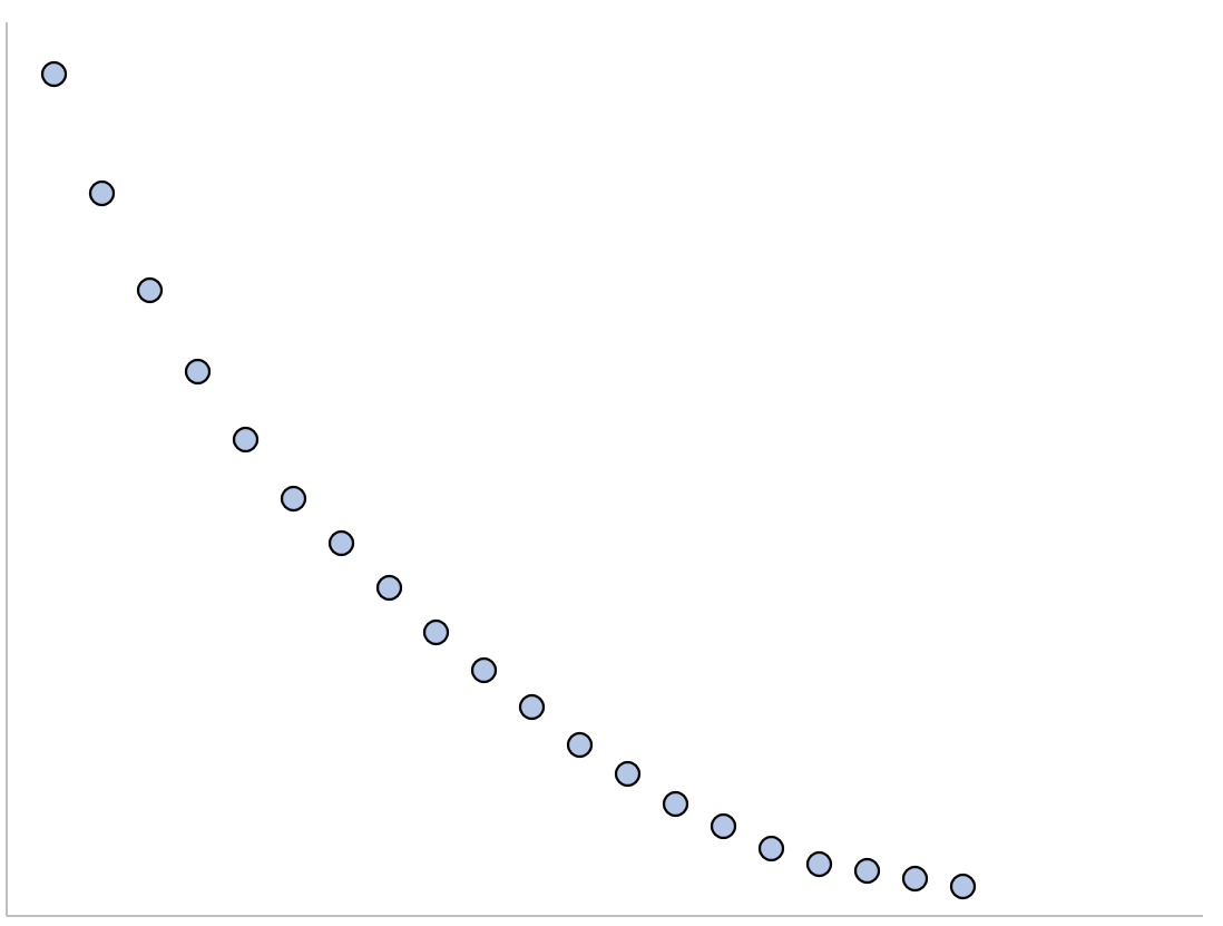
For this type of situation, the relationship between a predictor variable and a response variable could be modeled well using logarithmic regression.
The equation of a logarithmic regression model takes the following form:
y = a + b*ln(x)
where:
- y: The response variable
- x: The predictor variable
- a, b: The regression coefficients that describe the relationship between x and y
The following step-by-step example shows how to perform logarithmic regression in Python.
Step 1: Create the Data
First, let’s create some fake data for two variables: x and y:
import numpy as np
x = np.arange(1, 16, 1)
y = np.array([59, 50, 44, 38, 33, 28, 23, 20, 17, 15, 13, 12, 11, 10, 9.5])
Step 2: Visualize the Data
Next, let’s create a quick scatterplot to visualize the relationship between x and y:
import matplotlib.pyplot as plt

plt.scatter(x, y)
plt.show()
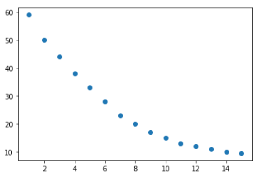
From the plot we can see that there exists a logarithmic decay pattern between the two variables. The value of the response variable, y, decreases rapidly at first and then slows over time.
Thus, it seems like a good idea to fit a logarithmic regression equation to describe the relationship between the variables.
Step 3: Fit the Logarithmic Regression Model
Next, we’ll use the polyfit() function to fit a logarithmic regression model, using the natural log of x as the predictor variable and y as the response variable:
#fit the model
fit = np.polyfit(np.log(x), y, 1)

#view the output of the model
print(fit)

[-20.19869943  63.06859979]
We can use the coefficients in the output to write the following fitted logarithmic regression equation:
y = 63.0686 – 20.1987 * ln(x)
We can use this equation to predict the response variable, y, based on the value of the predictor variable, x. For example, if x = 12, then we would predict that y would be 12.87:
y = 63.0686 – 20.1987 * ln(12) = 12.87
Bonus: Feel free to use this online Logarithmic Regression Calculator to automatically compute the logarithmic regression equation for a given predictor and response variable.
Additional Resources
A Complete Guide to Linear Regression in Python
How to Perform Exponential Regression in Python
How to Perform Logistic Regression in Python