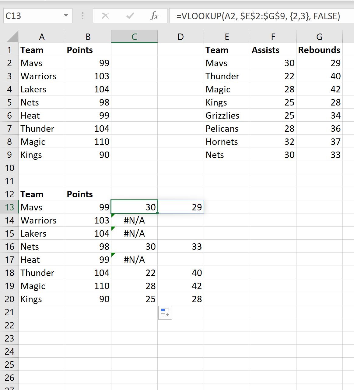
A left join allows you to join together two tables in which every row in the left table is kept and only the rows who have a matching value in a particular column of the right table are kept.
The following step-by-step example shows how to use the VLOOKUP function to perform a left join in Excel.
Step 1: Enter the Values for Each Table
First, let’s enter the following values for two tables in Excel:
We will perform a left join in which we keep all rows from the left table and only join in the rows from the right table that have matching values in the Team column.
Step 2: Create a Copy of the First Table
Next, let’s copy and paste the values of the first table into a new cell range:
Step 3: Perform Left Join Using VLOOKUP
Next, we’ll type the following formula into cell C13:
=VLOOKUP(A2, $E$2:$G$9, {2,3}, FALSE)
We’ll then drag and fill this formula down to each remaining cell in column C:
Feel free to add the column headers Assists and Rebounds as well:
The left join is now complete.
Each row from the left table is kept and only the rows with matching team names in the right table are kept.
If a given team didn’t have a match in the right table, then a #N/A value is shown for the Assists and Rebounds columns.
For example, the Mavs did exist in the right table, so they have corresponding values for Assists and Rebounds.
However, the Warriors did not exist in the right table, so they have #N/A for Assists and Rebounds.
Additional Resources
The following tutorials explain how to perform other common tasks in Excel:
Excel: How to Filter Cells that Contain Multiple Words
Excel: How to Filter a Column by Multiple Values
Excel Advanced Filter: Display Rows with Non-Blank Values


