Often you may have one or more missing values in a series in Excel that you’d like to fill in.
The simplest way to fill in missing values is to use the Fill Series function within the Editing section on the Home tab.
This tutorial provides two examples of how to use this function in practice.
Example 1: Fill in Missing Values for a Linear Trend
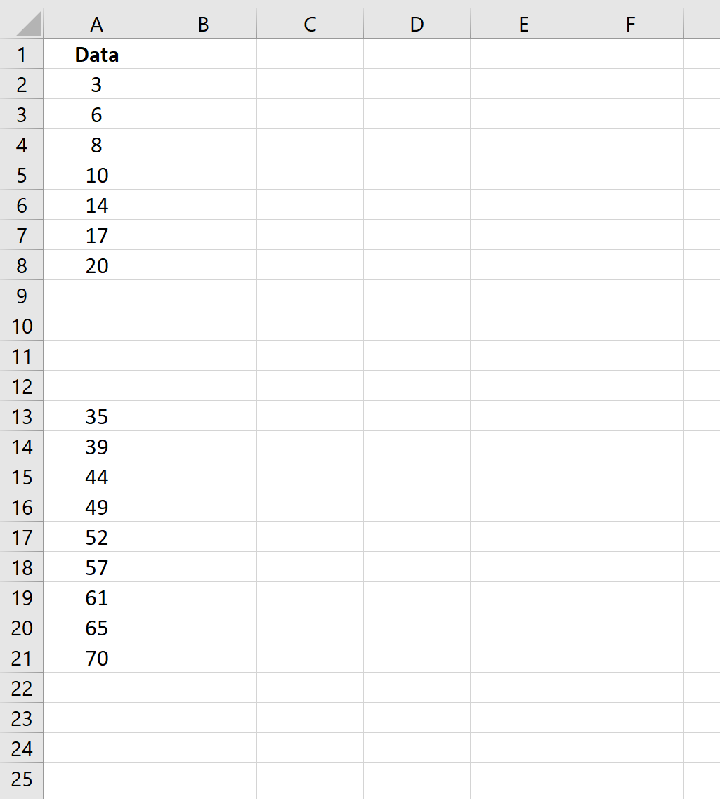
Suppose we have the following dataset with a few missing values in Excel:
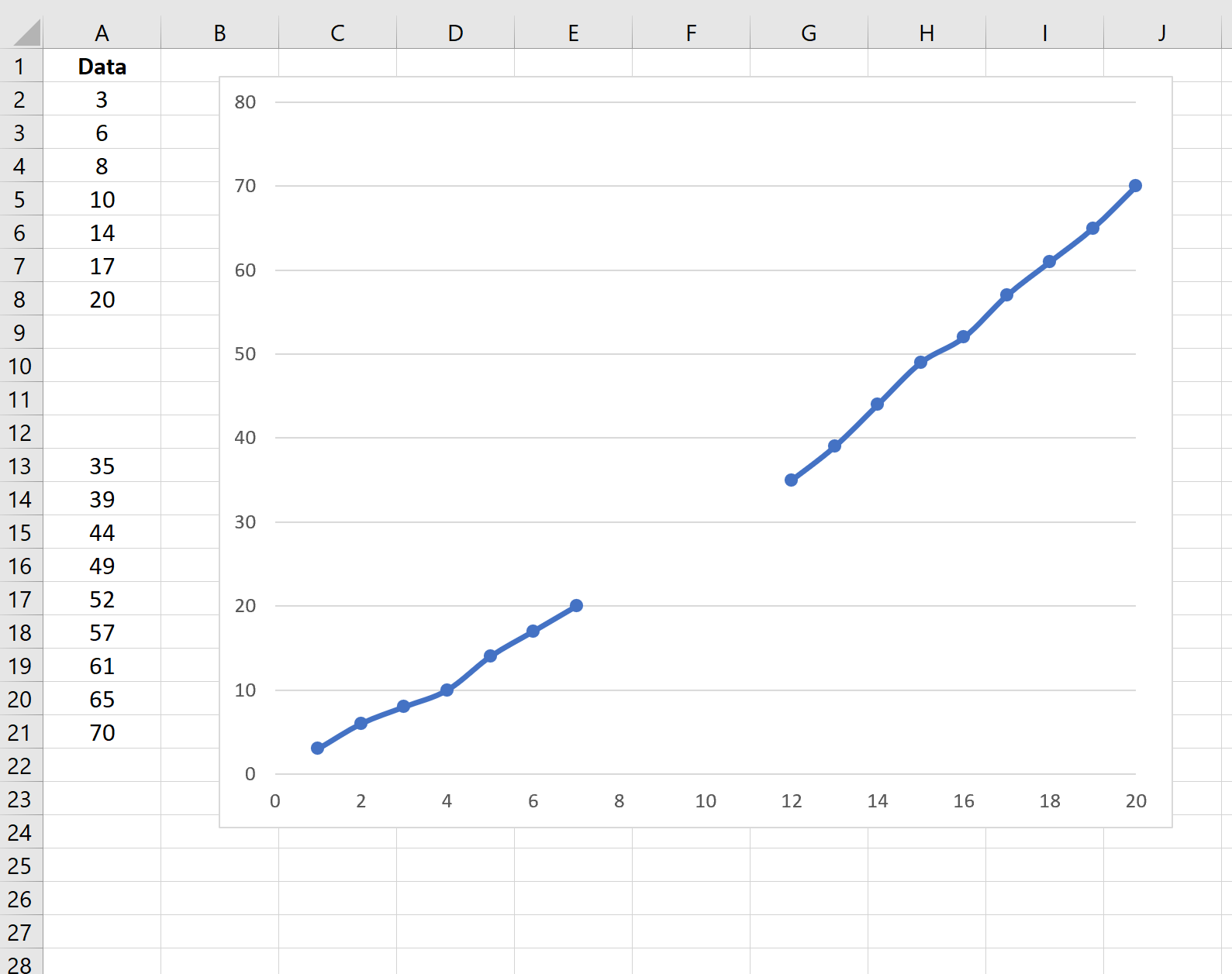
If we create a quick line chart of this data, we’ll see that the data appears to follow a linear trend:
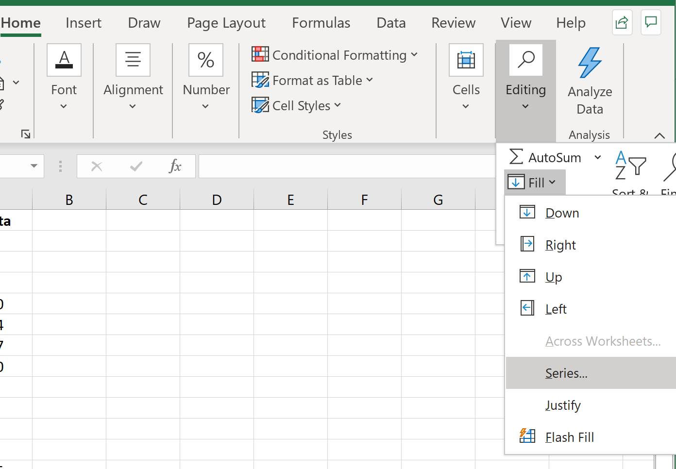
To fill in the missing values, we can highlight the range starting before and after the missing values, then click Home > Editing > Fill > Series.
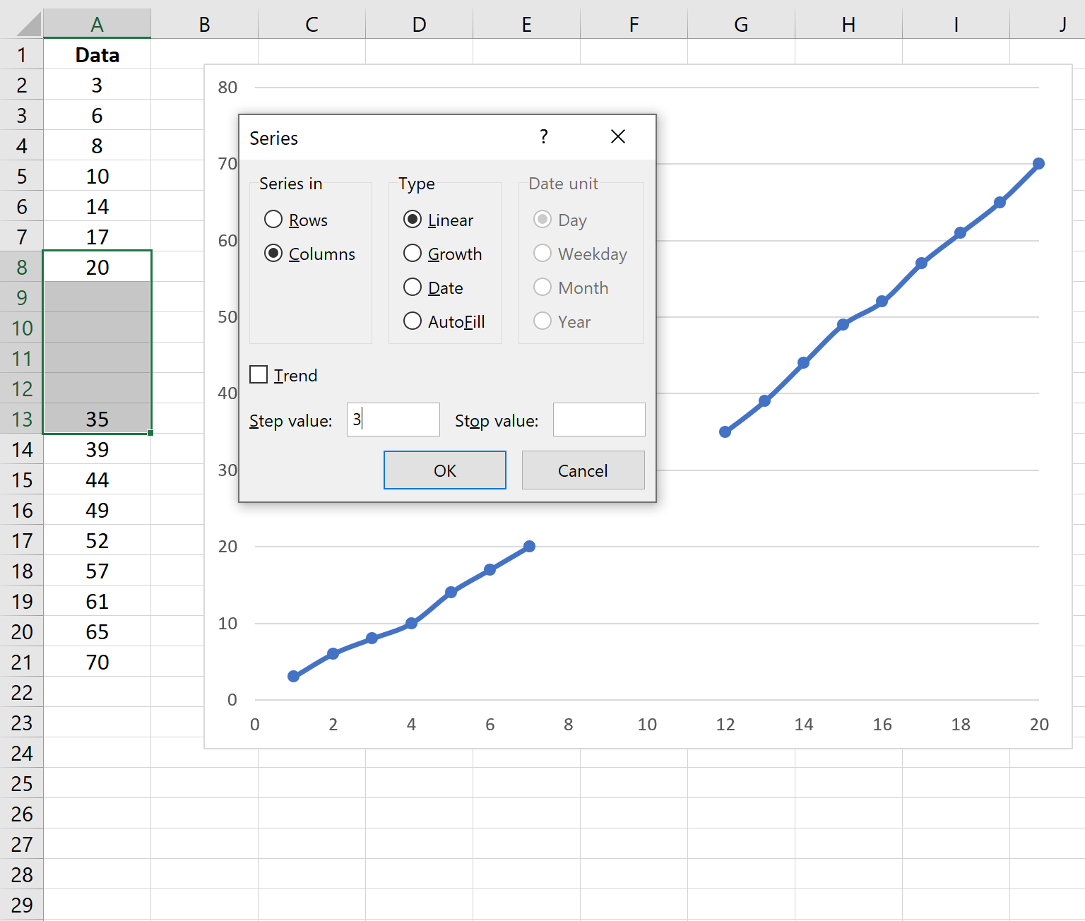
If we leave the Type as Linear, Excel will use the following formula to determine what step value to use to fill in the missing data:
Step = (End – Start) / (#Missing obs + 1)
For this example, it determines the step value to be: (35-20) / (4+1) = 3.
Once we click OK, Excel automatically fills in the missing values by adding 3 to the each subsequent value:

Example 2: Fill in Missing Values for a Growth Trend
Suppose we have the following dataset with a few missing values in Excel:
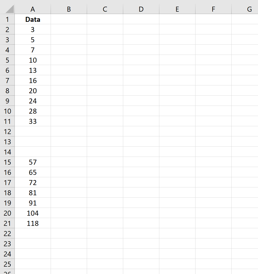
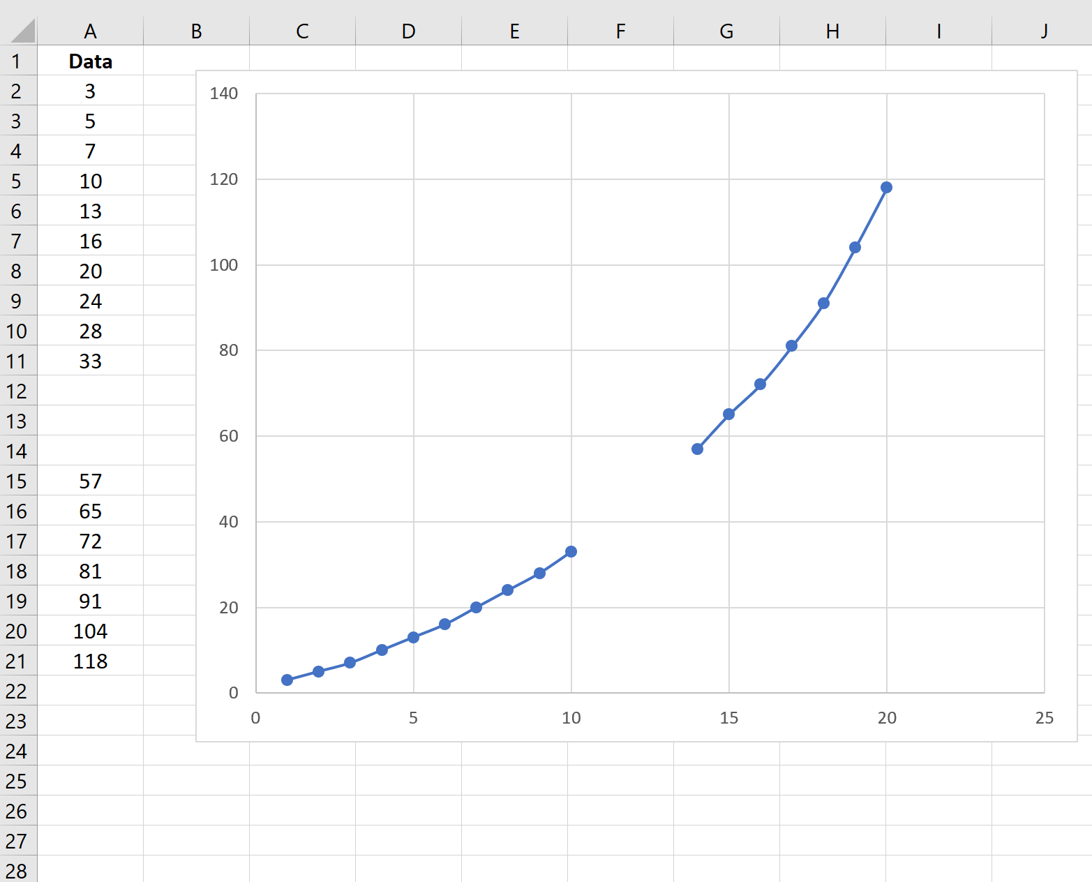
If we create a quick line chart of this data, we’ll see that the data appears to follow an exponential (or “growth”) trend:
To fill in the missing values, we can highlight the range starting before and after the missing values, then click Home > Editing > Fill > Series.

If we select the Type as Growth and click the box next to Trend, Excel automatically identifies the growth trend in the data and fills in the missing values.
Once we click OK, Excel fills in the missing values:
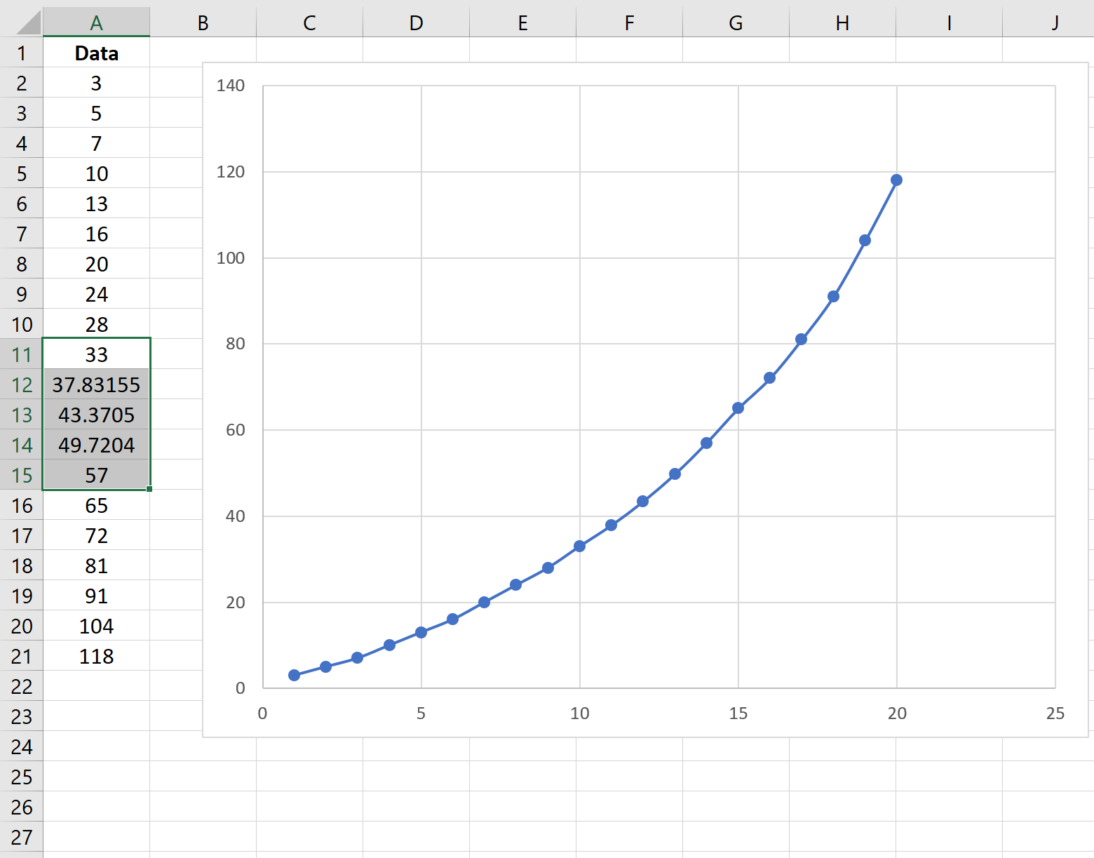
From the plot we can see that the filled-in values match the general trend of the data quite well.
You can find more Excel tutorials here.