You can use the following basic formula with INDEX and MATCH to return multiple values vertically in Excel:
=IFERROR(INDEX($B$2:$B$11,SMALL(IF($D$2=$A$2:$A$11,ROW($A$2:$A$11)-ROW($A$2)+1),ROW(1:1))),"")
This particular formula returns all of the values in the range B2:B11 where the corresponding value in the range A2:A11 is equal to the value in cell D2.
The following example shows how to use this formula in practice.
Example: Use INDEX and MATCH to Return Multiple Values Vertically
Suppose we have the following dataset in Excel that shows the name and team of various basketball players:
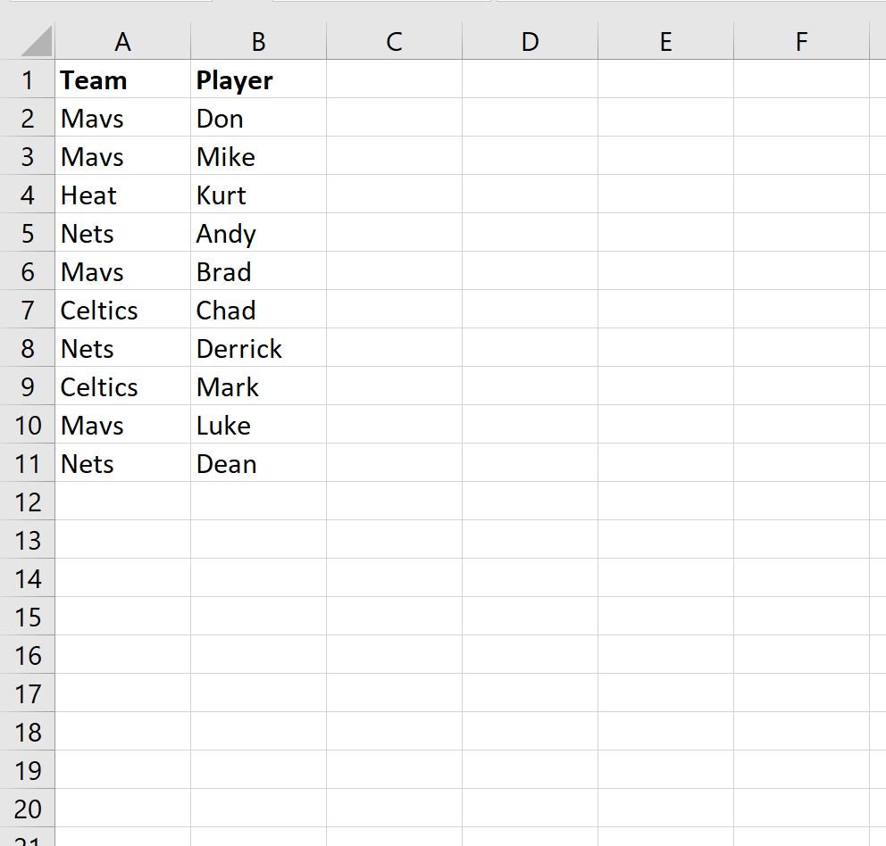
Now suppose we would like to return the names of each player who is on the Mavs team.
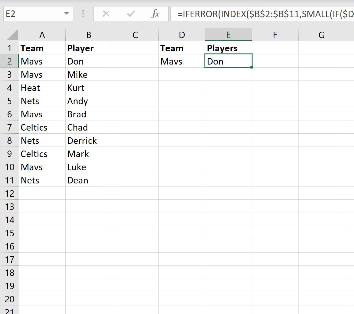
To do so, we can type the following formula into cell E2:
=IFERROR(INDEX($B$2:$B$11,SMALL(IF($D$2=$A$2:$A$11,ROW($A$2:$A$11)-ROW($A$2)+1),ROW(1:1))),"")
Once we press Enter, the name of the first player on the Mavs team will be returned:
We can then drag and fill this formula down to the remaining cells in column E to display the names of each player on the Mavs team:
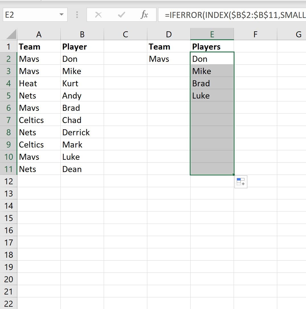
Notice that the names of each of the four players on the Mavs team are now shown.
Note that if you change the name of the team in cell D2, the names of the players shown in column E will change accordingly:
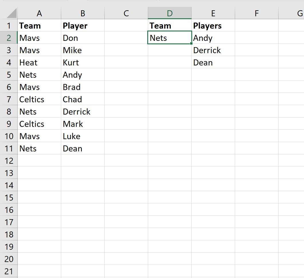
The names of each of the three players on the Nets team are now shown.
Additional Resources
The following tutorials explain how to perform other common tasks in Excel:
Excel: How to Perform a VLOOKUP with Two Lookup Values
Excel: How to Use VLOOKUP to Return Multiple Columns
Excel: How to Use VLOOKUP to Return All Matches