The residual standard error is used to measure how well a regression model fits a dataset.
In simple terms, it measures the standard deviation of the residuals in a regression model.
It is calculated as:
Residual standard error = √Σ(y – ŷ)2/df
where:
- y: The observed value
- ŷ: The predicted value
- df: The degrees of freedom, calculated as the total number of observations – total number of model parameters.
The smaller the residual standard error, the better a regression model fits a dataset. Conversely, the higher the residual standard error, the worse a regression model fits a dataset.
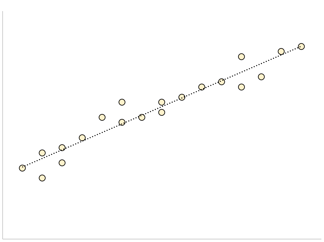
A regression model that has a small residual standard error will have data points that are closely packed around the fitted regression line:
The residuals of this model (the difference between the observed values and the predicted values) will be small, which means the residual standard error will also be small.
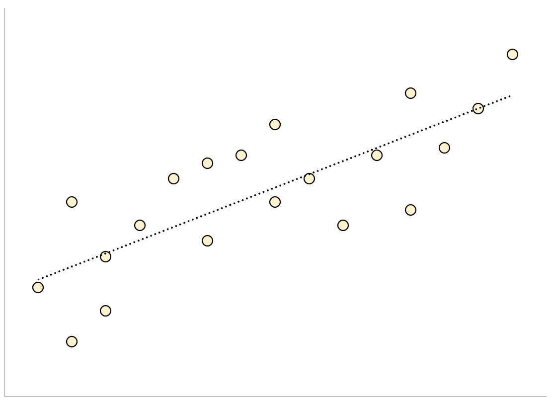
Conversely, a regression model that has a large residual standard error will have data points that are more loosely scattered around the fitted regression line:
The residuals of this model will be larger, which means the residual standard error will also be larger.
The following example shows how to calculate and interpret the residual standard error of a regression model in R.
Example: Interpreting Residual Standard Error
Suppose we would like to fit the following multiple linear regression model:
mpg = β0 + β1(displacement) + β2(horsepower)
This model uses the predictor variables “displacement” and “horsepower” to predict the miles per gallon that a given car gets.
The following code shows how to fit this regression model in R:
#load built-in mtcars dataset
data(mtcars)

#fit regression model
model #view model summary
summary(model)

Call:
lm(formula = mpg ~ disp + hp, data = mtcars)

Residuals:
    Min      1Q  Median      3Q     Max
-4.7945 -2.3036 -0.8246  1.8582  6.9363

Coefficients:
             Estimate Std. Error t value Pr(>|t|)
(Intercept) 30.735904   1.331566  23.083  3.127 on 29 degrees of freedom
Multiple R-squared:  0.7482,	Adjusted R-squared:  0.7309
F-statistic: 43.09 on 2 and 29 DF,  p-value: 2.062e-09
Near the bottom of the output we can see that the residual standard error of this model is 3.127.
This tells us that the regression model predicts the mpg of cars with an average error of about 3.127.
Using Residual Standard Error to Compare Models
The residual standard error is particularly useful for comparing the fit of different regression models.
For example, suppose we fit two different regression models to predict the mpg of cars. The residual standard error of each model is as follows:
- Residual standard error of model 1: 3.127
- Residual standard error of model 2: 5.657
Since model 1 has a lower residual standard error, it fits the data better than model 2. Thus, we would prefer to use model 1 to predict the mpg of cars because the predictions it makes are closer to the observed mpg values of the cars.
Additional Resources
How to Perform Simple Linear Regression in R
How to Perform Multiple Linear Regression in R
How to Create a Residual Plot in R


