You can use one of the following methods to calculate a weighted average in Google Sheets:
Method 1: Use AVERAGE.WEIGHTED
=AVERAGE.WEIGHTED(B2:B5, C2:C5)
Method 2: Use SUMPRODUCT
=SUMPRODUCT(B2:B5, C2:C5)/SUM(C2:C5)
Both formulas assume the values are in the range B2:B5 and the weights are in the range C2:C5.
Both formulas will return the same results, but the AVERAGE.WEIGHTED method requires less typing.
The following examples show how to use each formula in practice with the following dataset in Google Sheets:

Example 1: Calculate Weighted Average Using AVERAGE.WEIGHTED
We can type the following formula into cell E2 to calculate the weighted average of exam scores for this particular student:
=AVERAGE.WEIGHTED(B2:B5, C2:C5)
The following screenshot shows how to use this formula in practice:

From the output we can see that the weighted average of exam scores is 79.5.
Here’s how the AVERAGE.WEIGHTED formula actually calculated this value:
Weighted Average = (90*.15 + 80*.15 + 85*.15 + 75*.55) / (.15 + .15 + .15 + .55) = 79.5.
Example 2: Calculate Weighted Average Using SUMPRODUCT
We could also type the following formula into cell E2 to calculate the weighted average of exam scores for this particular student:
=SUMPRODUCT(B2:B5, C2:C5)/SUM(C2:C5)
The following screenshot shows how to use this formula in practice:
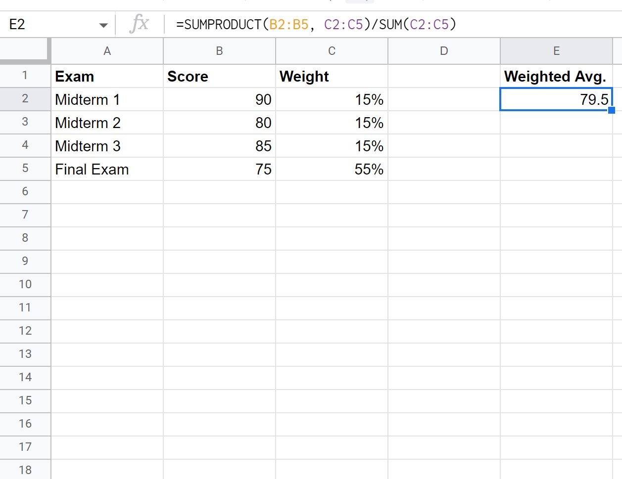
From the output we can see that the weighted average of exam scores is 79.5.
This matches the weighted average that we calculated in the previous example.
Additional Resources
The following tutorials explain how to perform other common operations in Google Sheets:
How to Calculate Average If Cell Contains Text in Google Sheets
How to Calculate Average by Month in Google Sheets
How to Average Filtered Rows in Google Sheets