The following step-by-step example shows how to display the percentage of a total in a pivot table in Google Sheets.
Step 1: Enter the Data
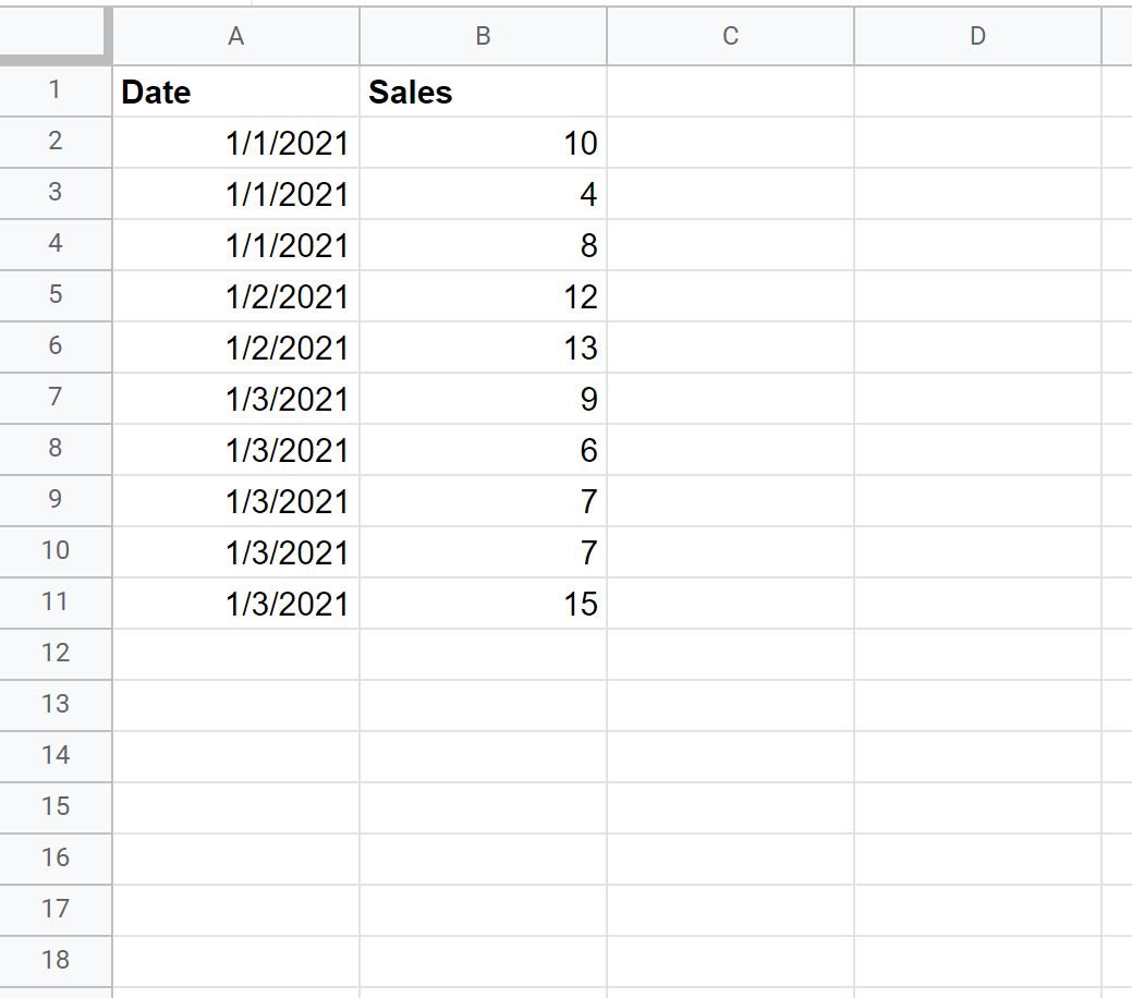
First, let’s enter the following data that shows the number of sales made during various days by some company:
Step 2: Create the Pivot Table
To create a pivot table that summarizes the total sales by day, click the Insert tab and then click Pivot table:

In the window that appears, type in the range of the data to use for the pivot table and select a cell in the existing sheet to place the pivot table:

Once you click Create, an empty pivot table will automatically be inserted.
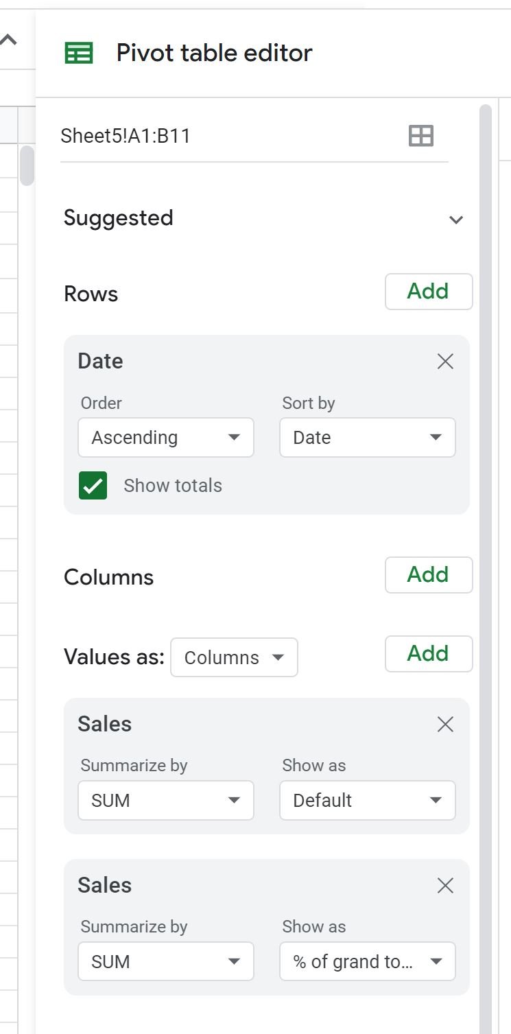
In the Pivot table editor that appears on the right side of the screen, perform the following actions:
- Click Add next to Rows and choose Date.
- Then click Add next to Values and click Sales.
- Then click Add next to Values and click Sales again.
- Then click the dropdown menu under Show as in the second Sales field and choose % of grand total:
The pivot table will automatically be populated with the following values:
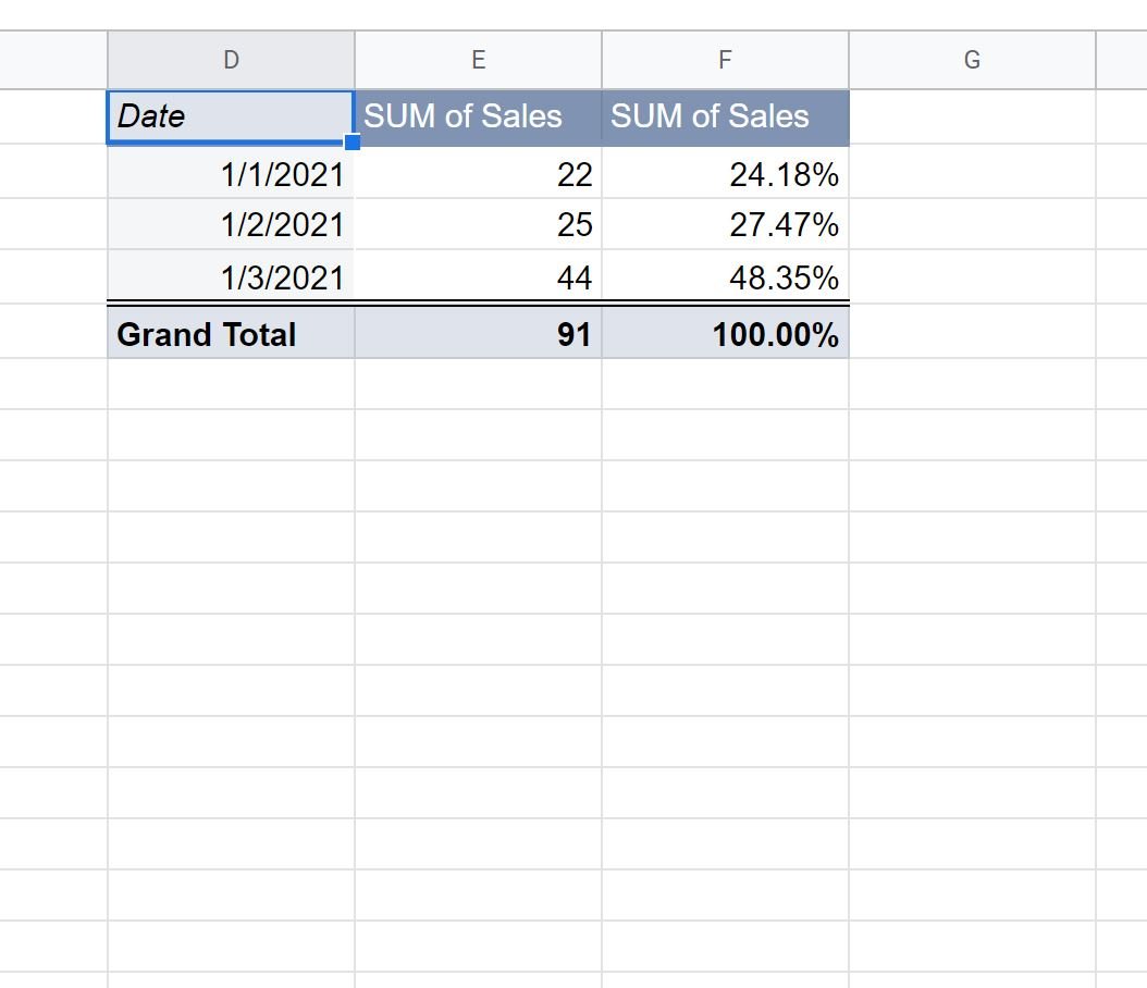
Here’s how to interpret the values in the pivot table:
- Column D shows the date.
- Column E shows the sum of sales for each date.
- Column F shows the percentage of total sales for each date.
In column F we can see:
- 24.18% of all sales were made on 1/1/2021.
- 27.47% of all sales were made on 1/2/2021.
- 48.35% of all sales were made on 1/3/2021.
Notice that the percentages sum to 100%.
Additional Resources
The following tutorials explain how to perform other common operations in Google Sheets:
How to Format Pivot Tables in Google Sheets
How to Add Calculated Field in Pivot Table in Google Sheets
How to Create a Pivot Table Using Google Sheets Query