You can use the following formulas to check if cells in a range are blank in Google Sheets:
Method 1: Check if All Cells in Range Are Blank
=AND(ARRAYFORMULA(ISBLANK(A2:C2)))
If all cells in the range A2:C2 are blank, this formula returns TRUE. Otherwise, it returns FALSE.
Method 2: Check if Any Cells in Range Are Blank
=OR(ARRAYFORMULA(ISBLANK(A2:C2)))
If any cells in the range A2:C2 are blank, this formula returns TRUE. Otherwise, it returns FALSE.
The following examples show how to use each method in Google Sheets.
Example 1: Check if All Cells in Range Are Blank
Suppose we have the following dataset in Google Sheets that contains information about various basketball players:
![]()
We’ll type the following formula into cell D2 to check if every cell in row 2 is blank:
=AND(ARRAYFORMULA(ISBLANK(A2:C2)))
We’ll then copy and paste this formula down to every remaining cell in column D:
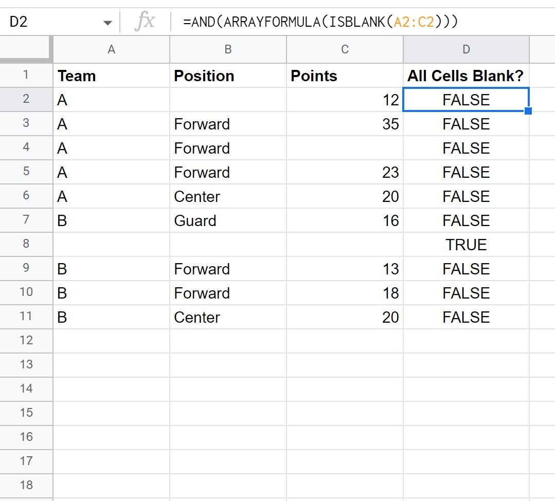
From the output we can see that the only row to return TRUE is row 8, which contains blank values in each column.
Example 2: Check if Any Cells in Range Are Blank
Once again suppose we have the following dataset in Google Sheets:
![]()
We’ll type the following formula into cell D2 to check if any cell in row 2 is blank:
=OR(ARRAYFORMULA(ISBLANK(A2:C2)))
We’ll then copy and paste this formula down to every remaining cell in column D:
![]()
From the output we can see that three rows return a value of TRUE.
Each of these rows has at least one blank cell.
Note: You can find the complete documentation for the ISBLANK function in Google Sheets here.
Additional Resources
The following tutorials explain how to perform other common tasks in Google Sheets:
How to Use “If Contains” in Google Sheets
How to Use ISERROR in Google Sheets
How to Ignore #N/A Values with Formulas in Google Sheets