You can use the following basic syntax with IMPORTRANGE in Google Sheets to import data from multiple spreadsheets at once:
=QUERY({
    IMPORTRANGE("URL1", "'sheetname1'!A1:B10");
    IMPORTRANGE("URL2", "'sheetname2'!A1:B10");
    IMPORTRANGE("URL3", "'sheetname3'!A1:B10");
  })
This particular query returns data from three different spreadsheets at once.
The following example shows how to use this syntax in practice.
Example: Use IMPORTRANGE with Multiple Sheets
Suppose we would like to import data from two different Google spreadsheets at once.
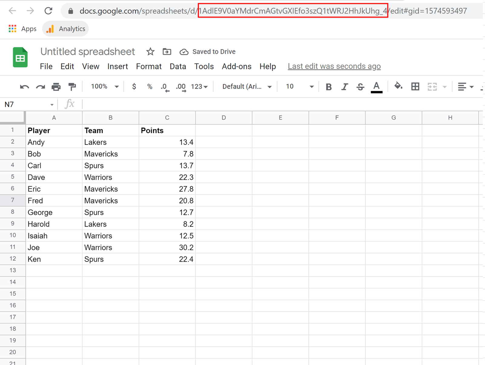
The first sheet is located in a tab called stats at the following URL:
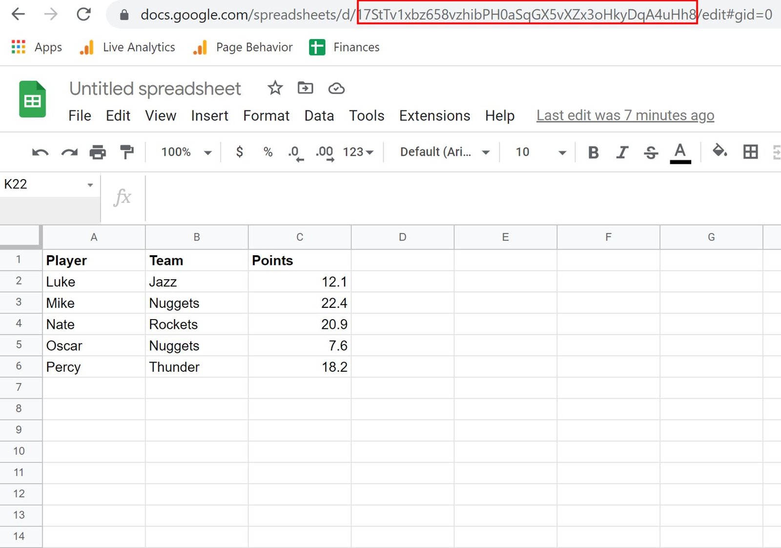
The second sheet is located in a tab called stats2 at the following URL:
We can use the following syntax with IMPORTRANGE to import the data from both sheets at once into a new spreadsheet:
=QUERY({IMPORTRANGE("1AdlE9V0aYMdrCmAGtvGXIEfo3szQ1tWRJ2HhJkUhg_4","'stats'!A1:C12");
        IMPORTRANGE("17StTv1xbz658vzhibPH0aSqGX5vXZx3oHkyDqA4uHh8","'stats2'!A1:C6")})
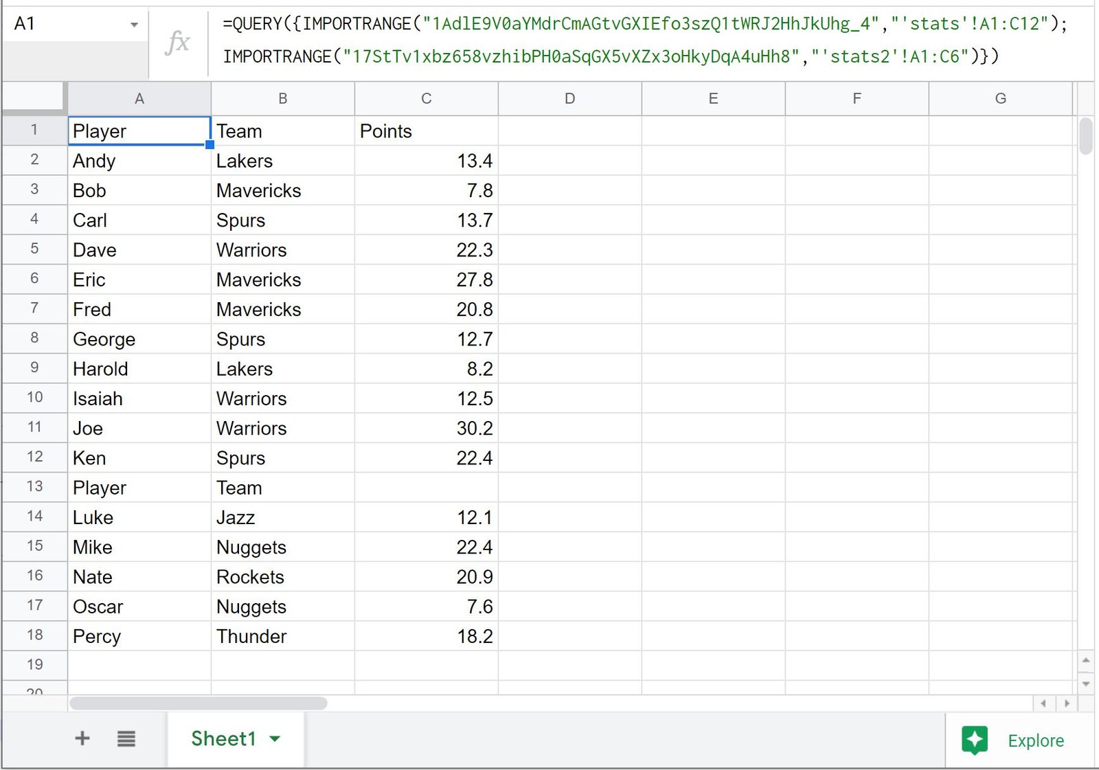
The following screenshot shows how to use this syntax in practice:
Notice that the data from both sheets is returned.
Also notice that the header column from the second sheet is returned in row 13.
To prevent this column from being imported, we can insert a where statement into our IMPORTRANGE function:
=QUERY({IMPORTRANGE("1AdlE9V0aYMdrCmAGtvGXIEfo3szQ1tWRJ2HhJkUhg_4","'stats'!A1:C12");
        IMPORTRANGE("17StTv1xbz658vzhibPH0aSqGX5vXZx3oHkyDqA4uHh8","'stats2'!A1:C6")},
        "where Col1!='Player'")
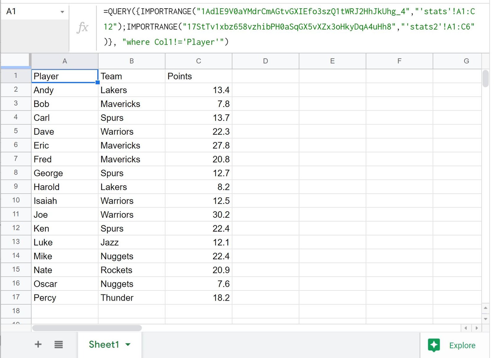
The following screenshot shows how to use this syntax in practice:
Notice that the data from both sheets is returned without the header row from the second sheet.
Additional Resources
The following tutorials explain how to perform other common tasks in Google Sheets:
Google Sheets: How to Query From Another Sheet
Google Sheets Query: How to Use Multiple Criteria in Query
Google Sheets Query: How to Return Only Unique Rows


