You can use the Conditional formatting option within the Format tab in Google Sheets to apply conditional formatting to cells if their date value is before today.
The following step-by-step example shows how to do so in practice.
Step 1: Enter the Data
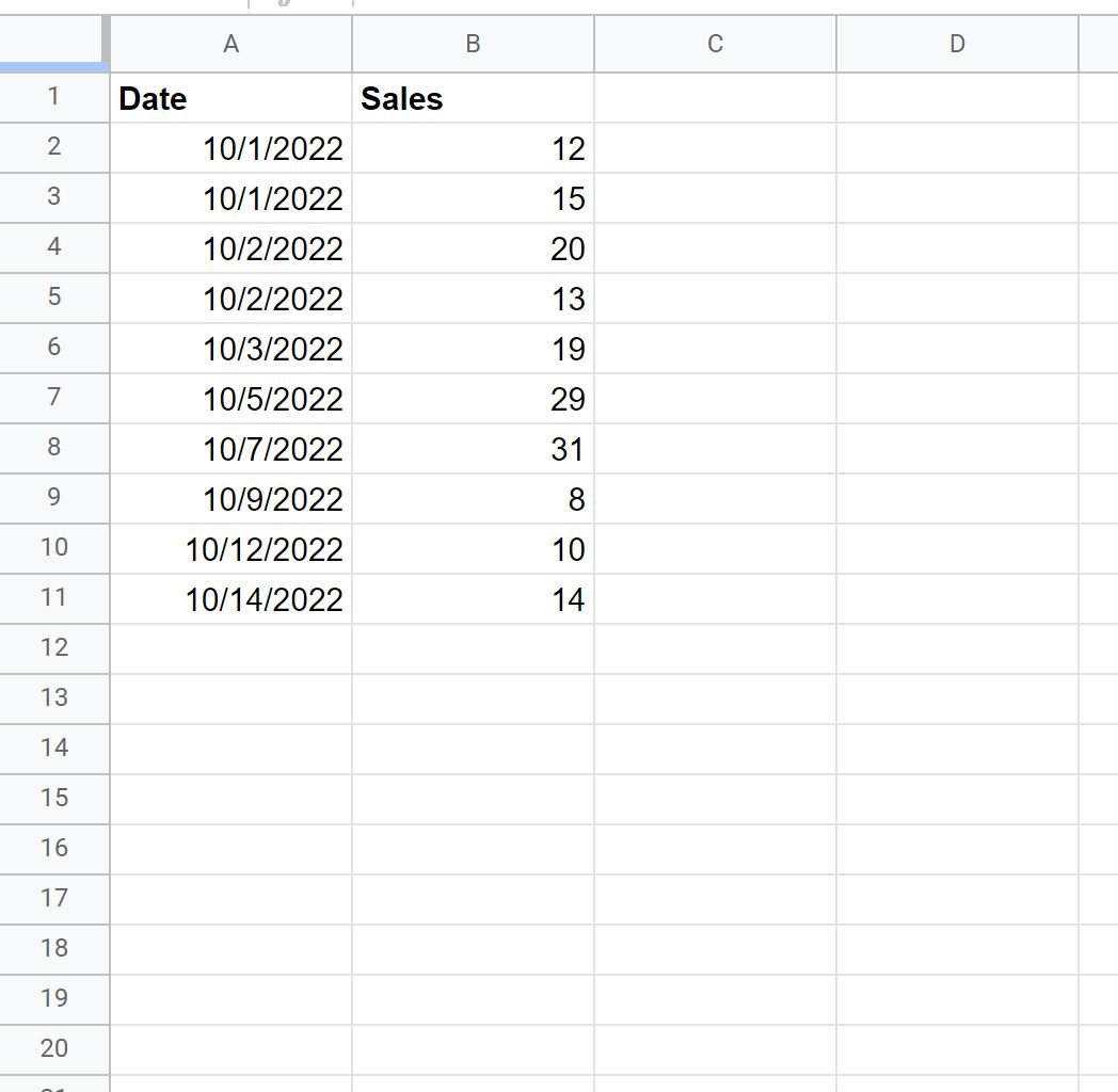
First, let’s enter the following dataset that shows the sales made at some retail store during various days:
Step 2: Apply Conditional Formatting to Cells if Date is Before Today
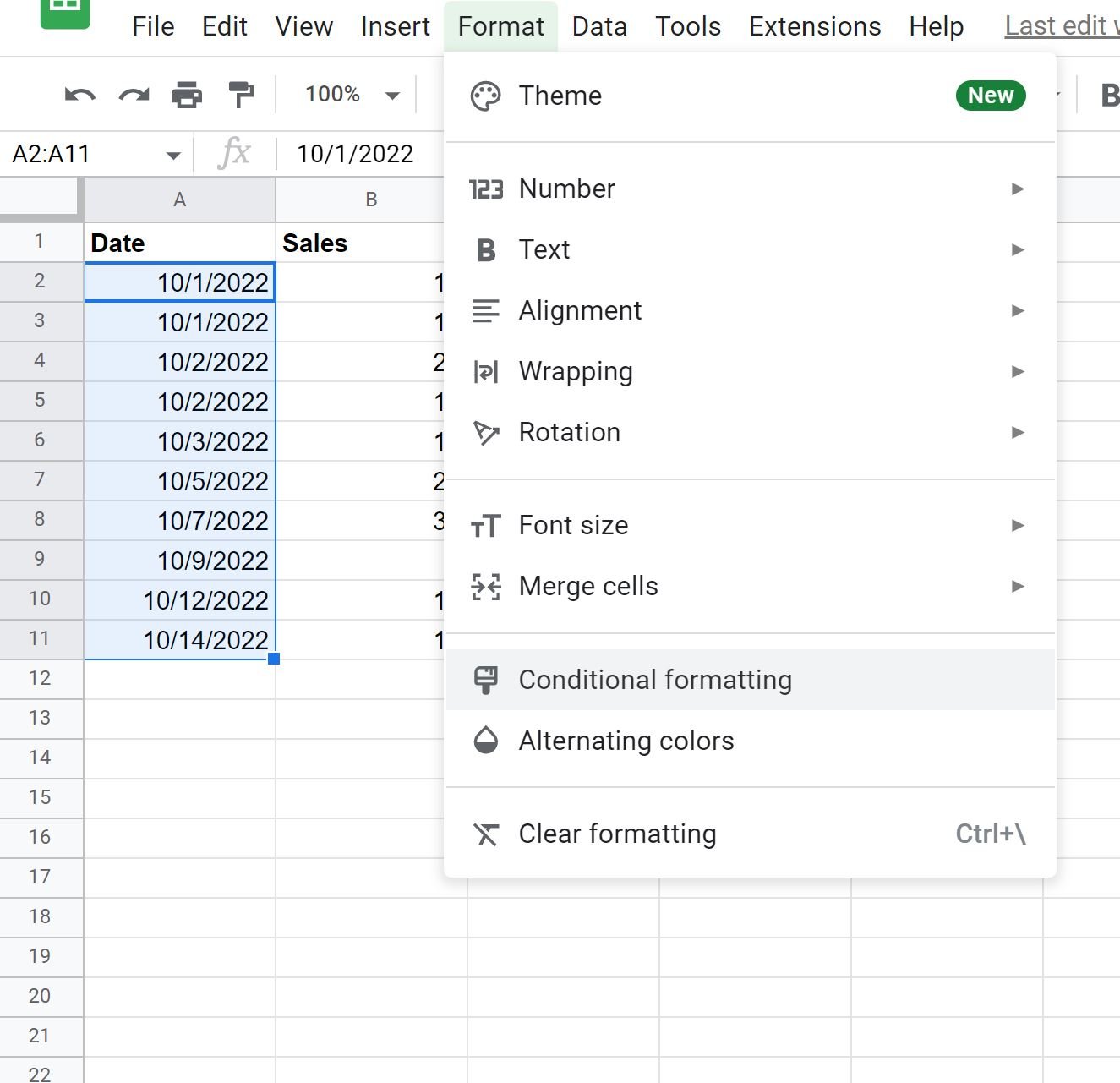
Next, highlight the cell range A2:A11, then click the Format tab, then click Conditional formatting:
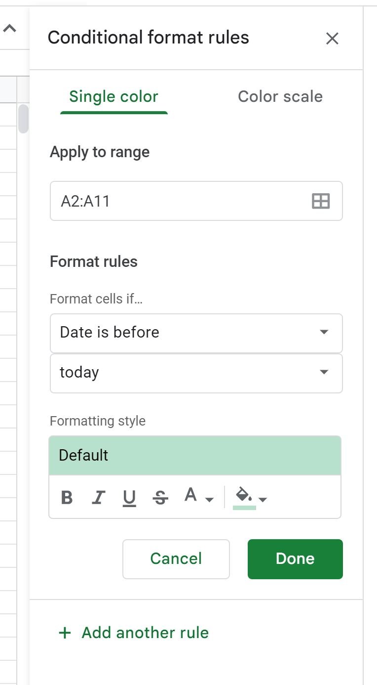
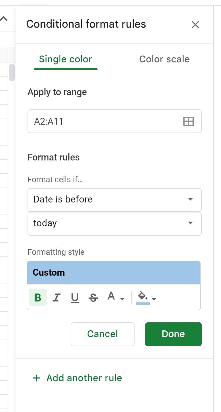
In the Conditional format rules panel that appears on the right side of the screen, click the dropdown menu under Format rules and choose Date is before, then choose today:
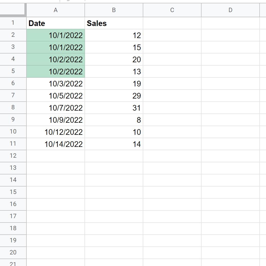
Assuming that today is 10/3/2022, all cells that are before this date will be highlighted:
Note that you can apply whatever conditional formatting rules you’d like to the cells that have a date before today.
For example, you might choose to make their font bold and their background light blue:
The formatting of the cells will automatically be changed:
Feel free to apply whatever conditional formatting you’d like.
Additional Resources
The following tutorials explain how to perform other common tasks in Google Sheets:
Google Sheets: A Simple Formula for “If Not Empty”
Google Sheets: A Simple Formula for “If Contains”
Google Sheets: How to Sum If Checkbox is Checked


