You can use the custom formula function in Google Sheets to apply conditional formatting to cells based on multiple conditions.
The following examples show how to use the custom formula function in the following scenarios:
1. Conditional Formatting with OR logic
2. Conditional Formatting with AND logic
Let’s jump in!
Example 1: Conditional Formatting with OR Logic
Suppose we have the following dataset in Google Sheets:
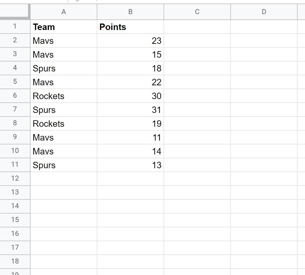
Suppose we’d like to highlight each of the cells in the Team column where the name is “Spurs” or “Rockets.”
To do so, we can highlight the cells in the range A2:A11, then click the Format tab, then click Conditional formatting:

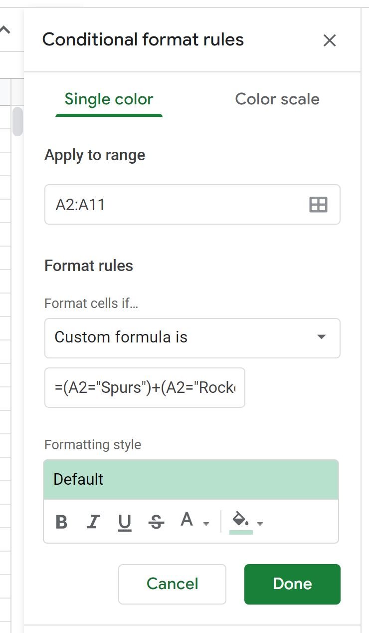
In the Conditional format rules panel that appears on the right side of the screen, click the Format cells if dropdown, then choose Custom formula is, then type in the following formula:
=(A2="Spurs")+(A2="Rockets")
Once you click Done, each of the cells in the Team column that are equal to “Spurs” or “Rockets” will automatically be highlighted:

Example 2: Conditional Formatting with AND Logic
Suppose we’d like to highlight each of the cells in the Team column where the name is “Spurs” and corresponding value in the Points column is greater than 15.
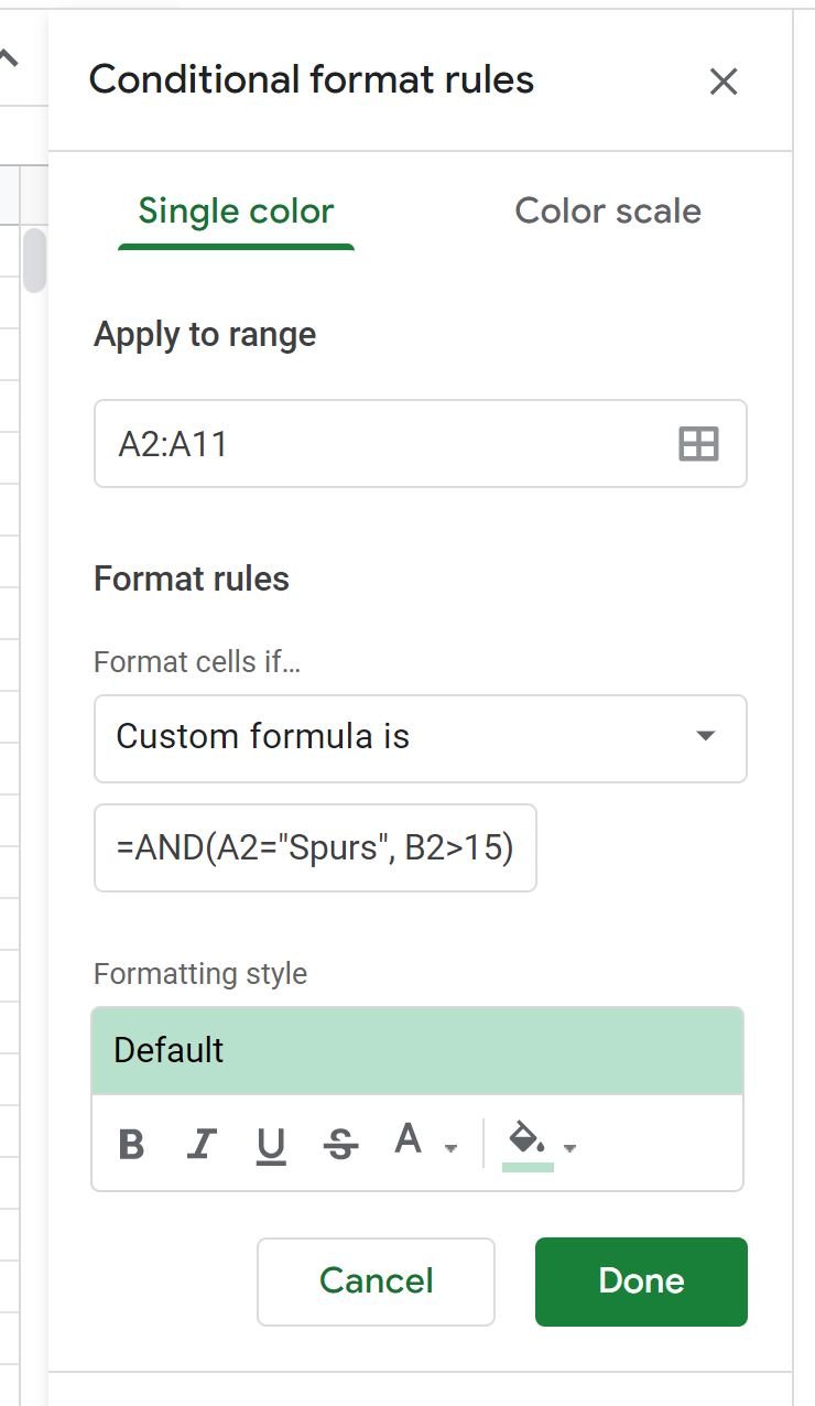
In the Conditional format rules panel, click the Format cells if dropdown, then choose Custom formula is, then type in the following formula:
=AND(A2="Spurs", B2>15)
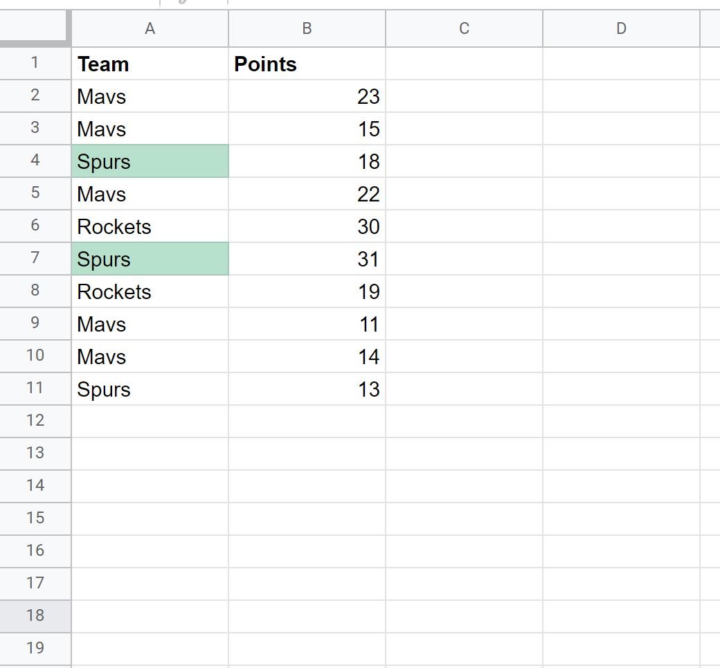
Once you click Done, each of the cells in the Team column that are equal to “Spurs” and where the corresponding value in the Points column is greater than 15 will automatically be highlighted:
Additional Resources
The following tutorials explain how to perform other common tasks in Google Sheets:
How to Replace Text in Google Sheets
How to Replace Blank Cells with Zero in Google Sheets
How to Use a Case Sensitive VLOOKUP in Google Sheets
Google Sheets: Conditional Formatting if Another Cell Contains Text