You can use the custom formula function in Google Sheets to apply conditional formatting based on a cell value from another sheet.
The following example shows how to use the custom formula function in practice.
Example: Conditional Formatting Based on Another Sheet
Suppose we have the following dataset in Sheet1 that shows the total points scored by various basketball teams:

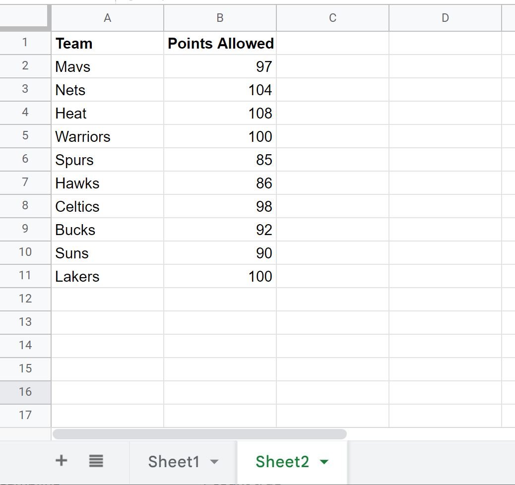
And suppose we have the following dataset in Sheet2 that shows the total points allowed by the same list of teams:
Suppose we’d like to highlight each of the cells in the Team column of Sheet1 if the value in the Points Scored column is greater than the value in the Points Allowed column in Sheet2.
To do so, we can highlight the cells in the range A2:A11, then click the Format tab, then click Conditional formatting:

In the Conditional format rules panel that appears on the right side of the screen, click the Format cells if dropdown, then choose Custom formula is, then type in the following formula:
=B2>INDIRECT("Sheet2!B2")
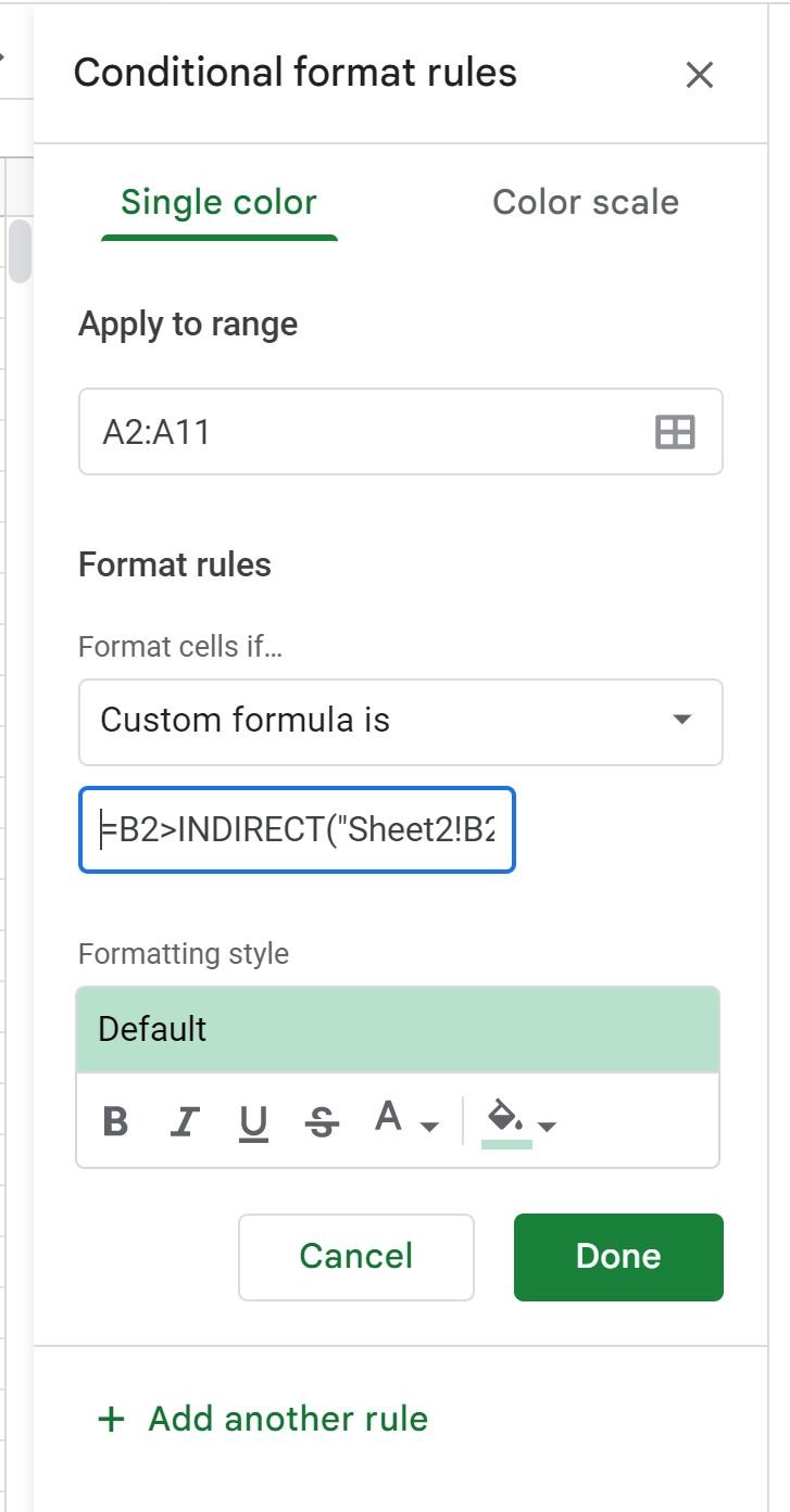
Note: It’s important that you include the equal sign (=) at the beginning of the formula, otherwise the conditional formatting won’t work.
Once you click Done, each of the cells in the Team column where the value in the Points Scored column is greater than the value in the Points Allowed column in Sheet2 will be highlighted with a green background:

The only Team values that have a green background are the ones where the value in the Points Scored column in Sheet1 is greater than the Points Allowed column in Sheet2.
Note that if the sheet name you’re referencing has spaces in the name, be sure to include single quotes around the sheet name.
For example, if your sheet is called Sheet 2 then you should use the following syntax when defining the formatting rule:
=B2>INDIRECT("'Sheet 2'!B2")
Additional Resources
The following tutorials explain how to perform other common tasks in Google Sheets:
Google Sheets: Conditional Formatting If Date is Before Today
Google Sheets: Conditional Formatting with Multiple Conditions
Google Sheets: Conditional Formatting if Another Cell Contains Text