How to Plot a Regression Line by Group with ggplot2

We can use the following syntax to plot a regression line by group using the R visualization package ggplot2:

ggplot(df, aes(x = x_variable, y = y_variable, color = group_variable)) +
  geom_point() +
  geom_smooth(method = "lm", fill = NA)

This tutorial provides a quick example of how to use this function in practice.

Example: Plot Regression Lines by Group with ggplot2

Suppose we have the following dataset that shows the following three variables for 15 different students:

• Number of hours studied
• Exam score received
• Study technique used (either A, B, or C)

#create dataset
df rep(c('A', 'B', 'C'), each=5))

#view dataset
df

   hours score technique
1      1    84         A
2      2    86         A
3      3    85         A
4      3    87         A
5      4    94         A
6      1    74         B
7      2    76         B
8      2    75         B
9      3    77         B
10     4    79         B
11     1    65         C
12     2    67         C
13     3    69         C
14     4    72         C
15     4    80         C

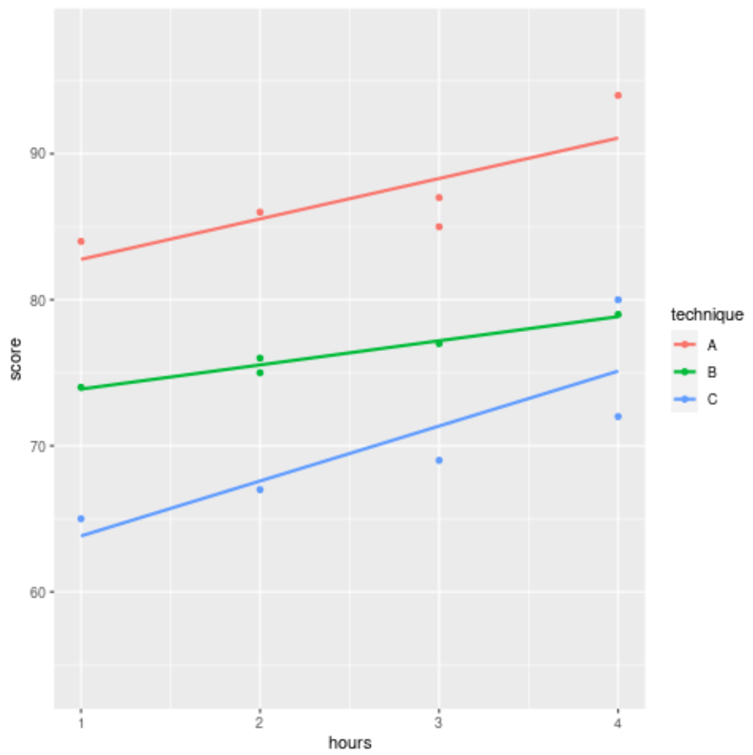
The following code shows how to plot a regression line that captures the relationship between hours studied and exam score received for each of the three study techniques:

#load ggplot2
library(ggplot2)

#create regression lines for all three groups
ggplot(df, aes(x = hours, y = score, color = technique)) +
  geom_point() +
  geom_smooth(method = "lm", fill = NA)

Note that in geom_smooth() we used method = ‘lm” to specify a linear trend.

We could also use other smoothing methods like “glm”, “loess”, or “gam” to capture nonlinear trends in the data. You can find the full documentation for geom_smooth() here.

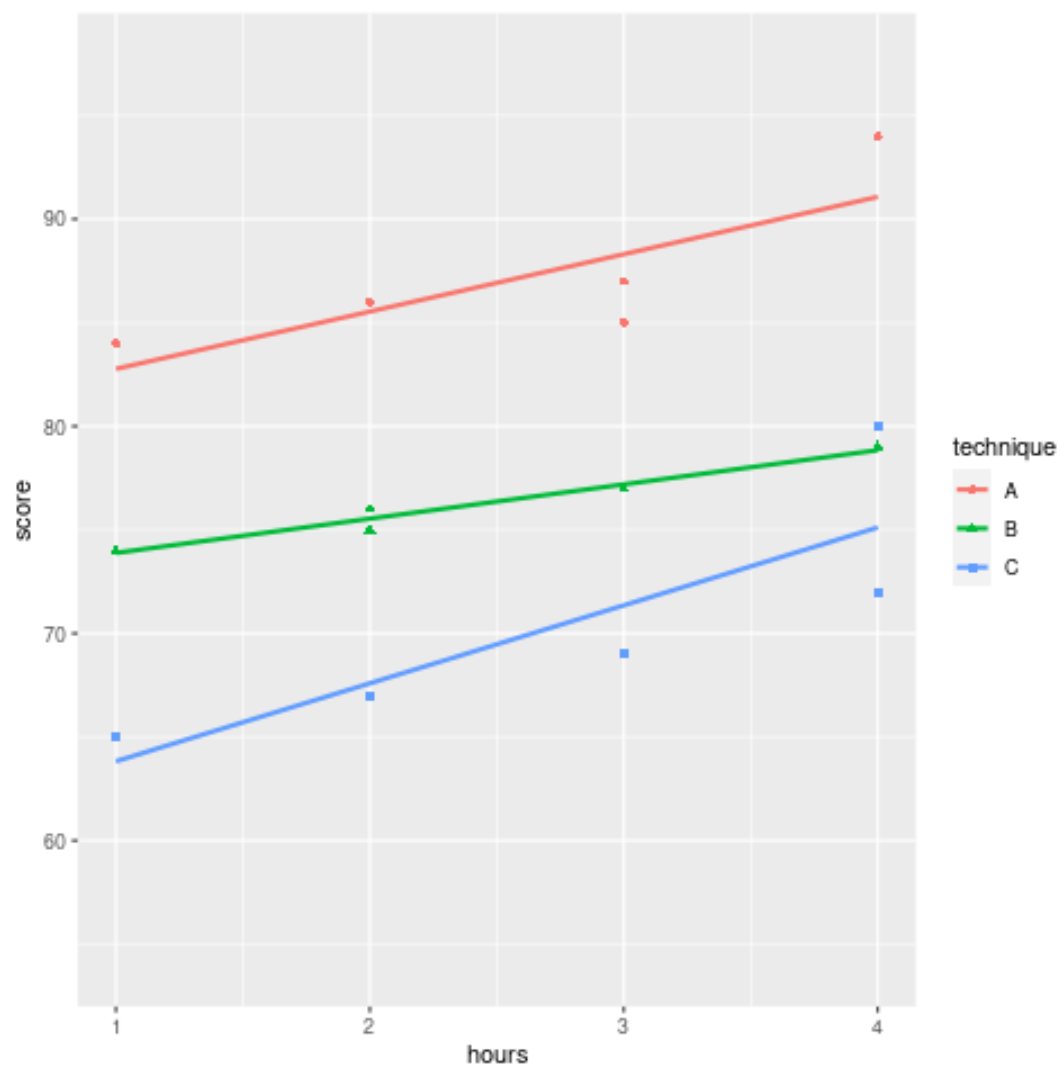
Note that we could also use different shapes to display the exam scores for each of the three groups:

ggplot(df, aes(x = hours, y = score, color = technique, shape = technique)) +
  geom_point() +
  geom_smooth(method = "lm", fill = NA)

You can find more ggplot2 tutorials here.