You can use the following formulas to find the top 10 values in Excel based on criteria:
Method 1: Find Top 10 Based on One Criteria
=LARGE(IF(A2:A20="Value",C2:C20,""),ROW(A1:A10))
This formula finds the top 10 values in the range C2:C20 where the value in the range A2:A20 is equal to “Value.”
Method 2: Find Top 10 Based on Multiple Criteria
=LARGE(IF((A2:A20="Value")*(--B2:B20>10),C2:C20,""),ROW(A1:A10))
This formula finds the top 10 values in the range C2:C20 where the value in the range A2:A20 is equal to “Value” and the value in the range B2:B20 is greater than 10.
The following examples show how to use each formula in practice.
Example 1: Find Top 10 Values Based on One Criteria
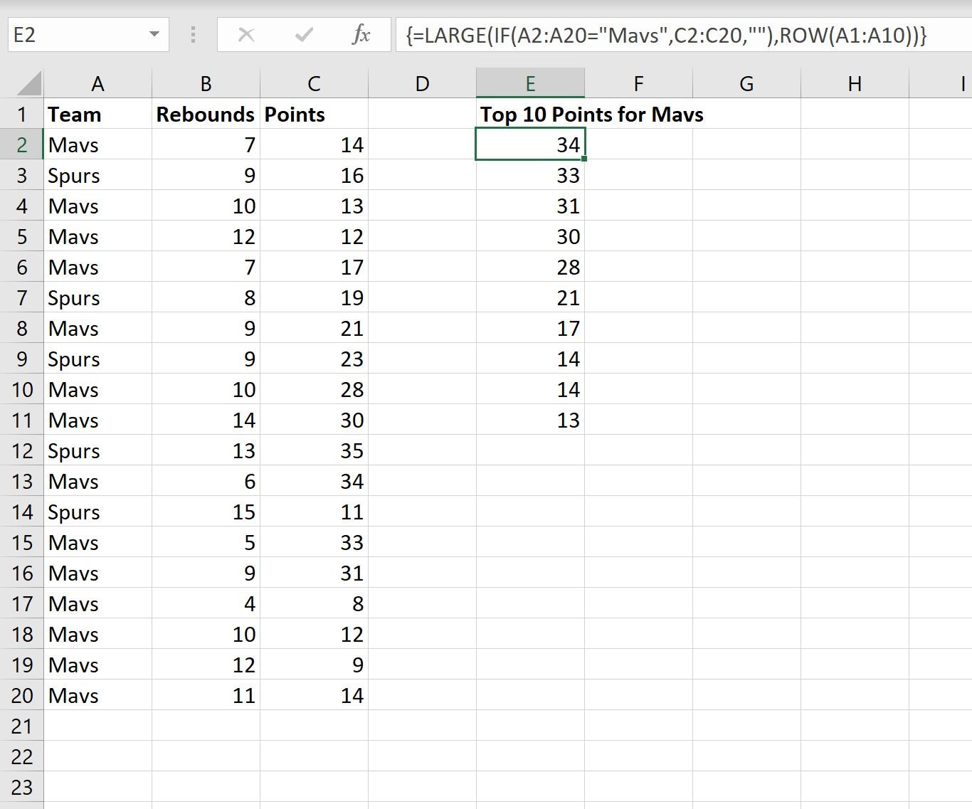
We can use the following formula to find the top 10 values in the Points column where the value in the Team column is equal to “Mavs”:
=LARGE(IF(A2:A20="Mavs",C2:C20,""),ROW(A1:A10))
Note: Make sure you press Ctrl+Shift+Enter after typing this formula.
The following screenshot shows how to use this formula in practice:
Column E shows the top 10 values from the Points column where the the Team column is equal to “Mavs.”
Example 2: Find Top 10 Values Based on Multiple Criteria
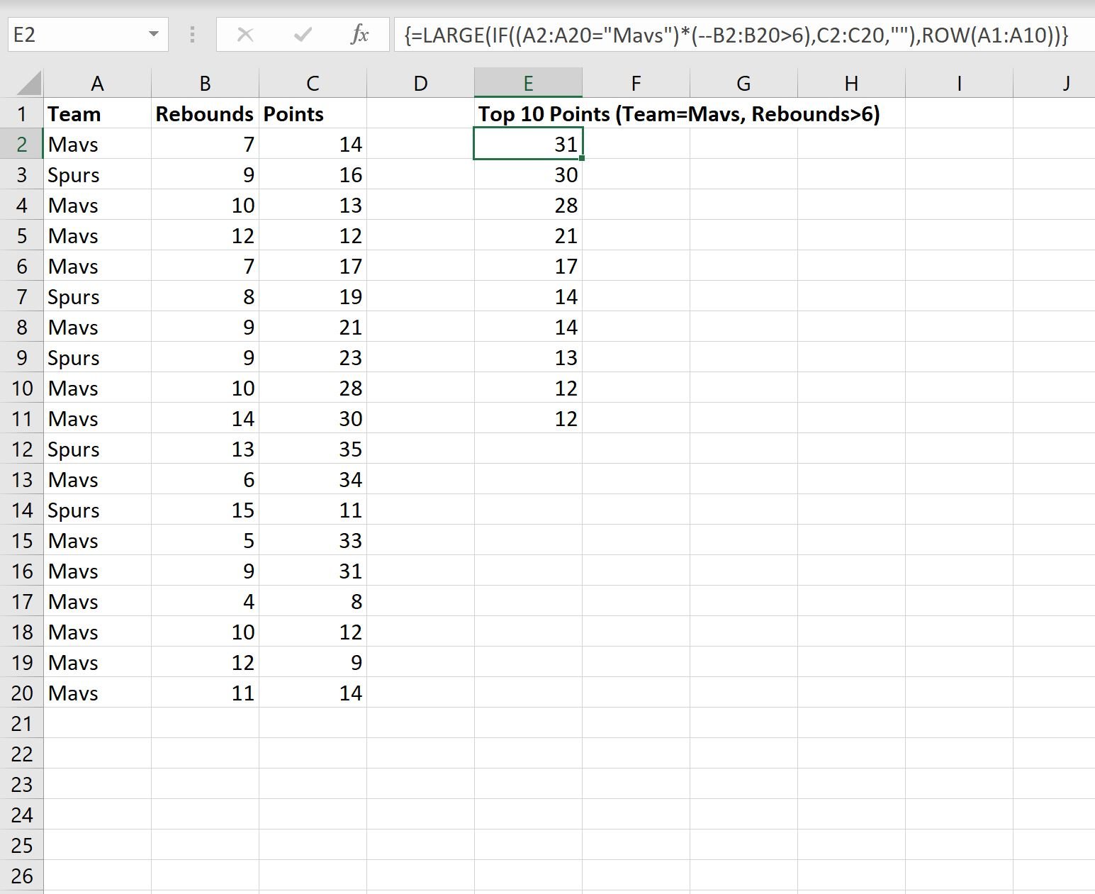
We can use the following formula to find the top 10 values in the Points column where the value in the Team column is equal to “Mavs” and the value in the Rebounds column is greater than 6:
=LARGE(IF((A2:A20="Mavs")*(--B2:B20>6),C2:C20,""),ROW(A1:A10))
Note: Make sure you press Ctrl+Shift+Enter after typing this formula.
The following screenshot shows how to use this formula in practice:
Column E shows the top 10 values from the Points column where the the Team column is equal to “Mavs” and the “Rebounds” column is greater than 6.
Additional Resources
The following tutorials explain how to perform other common tasks in Excel:
How to Calculate a Five Number Summary in Excel
How to Calculate the Mean and Standard Deviation in Excel
How to Calculate the Interquartile Range (IQR) in Excel


