The following step-by-step example shows how to sort an Excel pivot table by the grand total values.
Step 1: Enter the Data
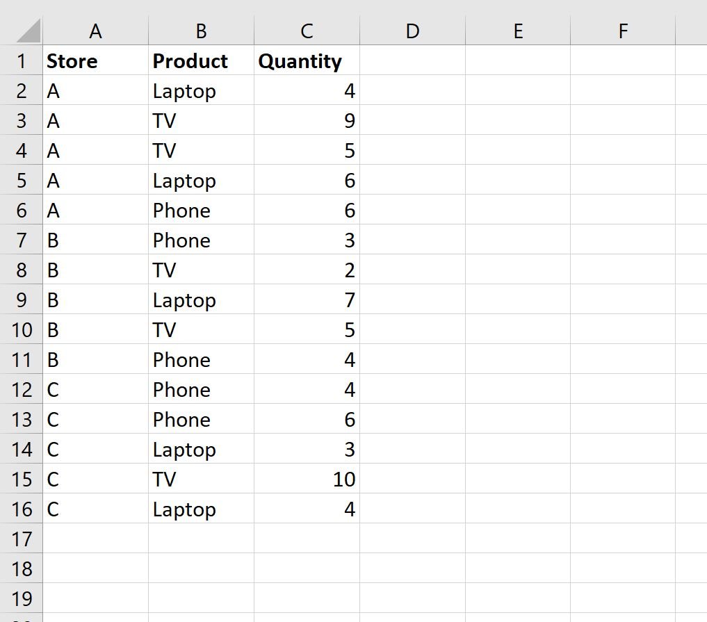
First, let’s enter the following sales data for three different stores:
Step 2: Create the Pivot Table
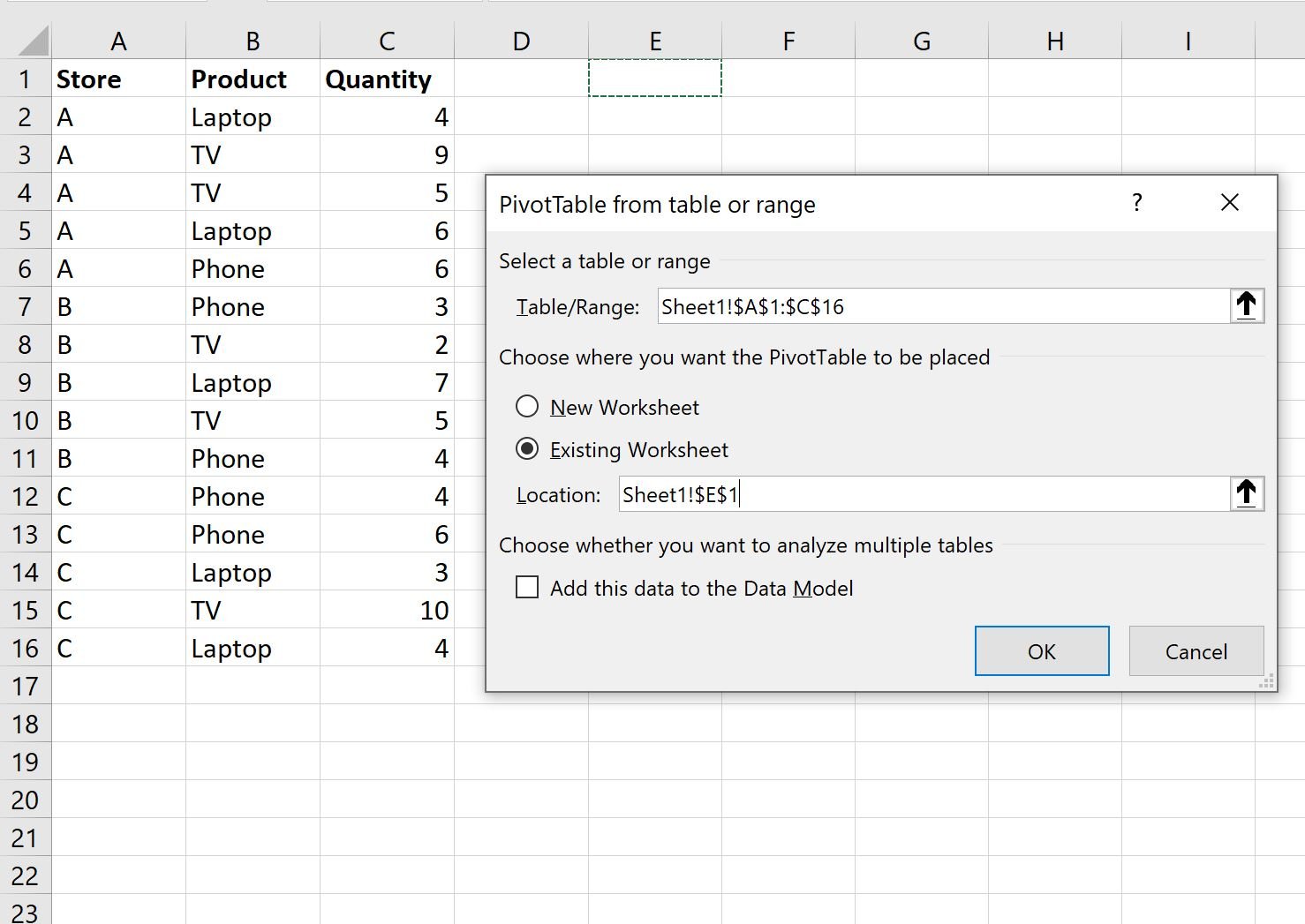
To create a pivot table, click the Insert tab along the top ribbon and then click the PivotTable icon:

In the new window that appears, choose A1:C16 as the range and choose to place the pivot table in cell E1 of the existing worksheet:
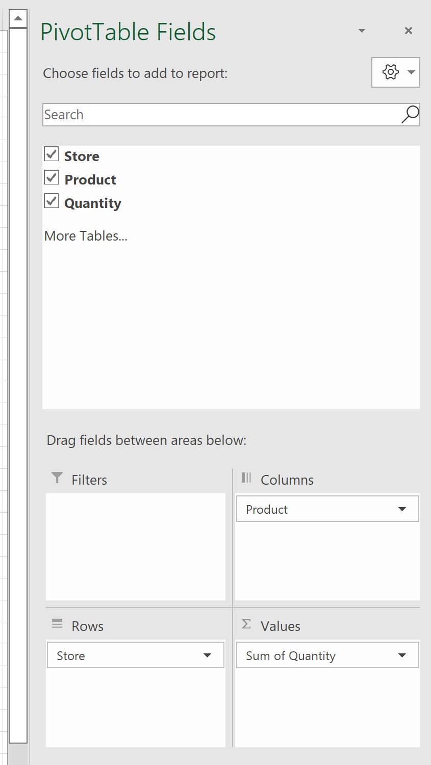
Once you click OK, a new PivotTable Fields panel will appear on the right side of the screen.
Drag the Store field to the Rows box, then drag the Product field to the Columns box, then drag the Quantity field to the Values box:
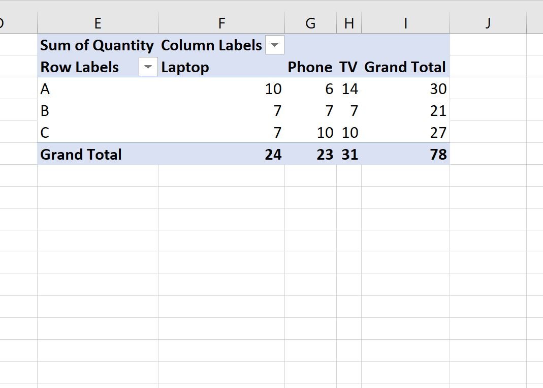
The pivot table will automatically be populated with the following values:
Step 3: Sort the Pivot Table by Grand Total
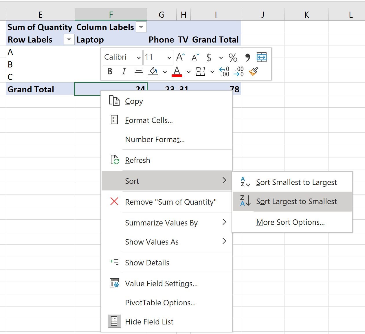
To sort the pivot table by the values in the last row titled Grand Total, simply right click on any of the values in the Grand Total row.
In the dropdown menu that appears, click Sort, then click Sort Largest to Smallest:
The columns of the pivot table will automatically be sorted from largest to smallest:
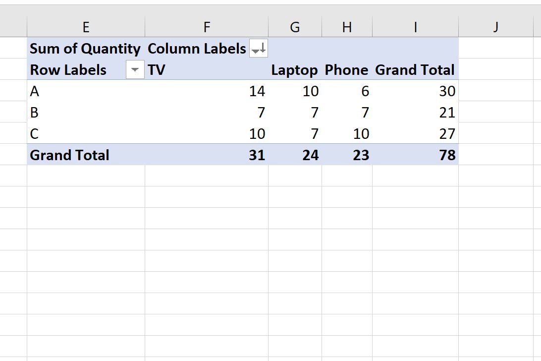
The TV column (31) is first, the Laptop column (24) is second, and the Phone column (23) is now third.
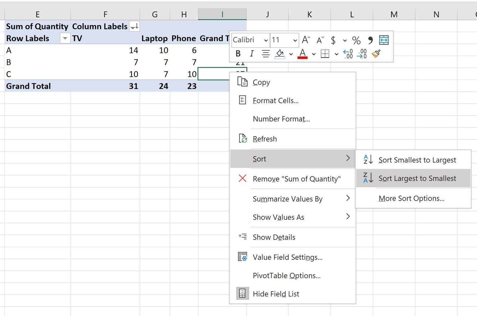
To instead sort the rows of the pivot table, right click on one of the values in the Grand Total column.
In the dropdown menu that appears, click Sort, then click Sort Largest to Smallest:
The rows of the pivot table will automatically be sorted from largest to smallest:
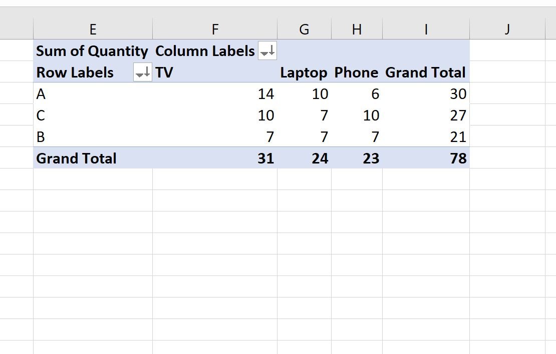
Store A (30) is first, store C (27) is second, and store B (21) is now third.
Additional Resources
The following tutorials explain how to perform other common tasks in Excel:
How to Create Tables in Excel
How to Group Values in Pivot Table by Range in Excel
How to Group by Month and Year in Pivot Table in Excel