You can use a combination of the RANK.EQ() function and the COUNTIFS() function in Excel to rank items by multiple criteria.
The following example shows how to use these functions to rank items in a list by multiple criteria in Excel.
Example: Rank by Multiple Criteria in Excel
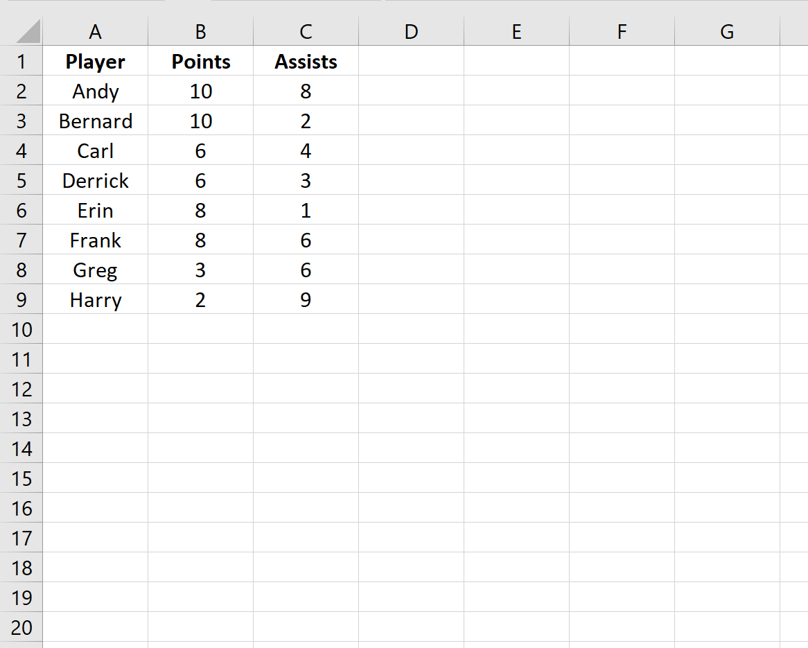
Suppose we have the following dataset in Excel that shows the total points and assists for eight different basketball players.
Now suppose we’d like to rank each player using the following criteria:
- First, rank each player based on points.
- Then, rank each player based on assists.
We can use the following formula to perform this multiple criteria ranking:
=RANK.EQ($B2, $B$2:$B$9) + COUNTIFS($B$2:$B$9, $B2, $C$2:$C$9, ">" &$C2)
We can type this formula into cell D2 of our spreadsheet, then copy and paste the formula down to every other cell in column D:
From the output we can see that Andy receives a rank of 1 because he is tied for the most points with Bernard. However, Andy has more assists than Bernard, so he receives a rank of 1 while Bernard receives a rank of 2.
Each player is ranked in a similar manner, first based on their total points and then based on their total assists.
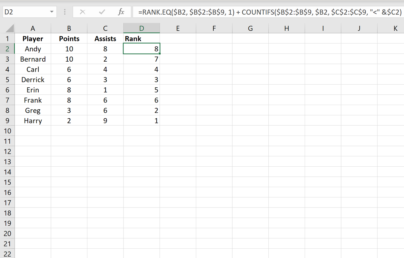
If we instead would like to perform multiple criteria ranking in reverse order (the “best” player gets the highest ranking) then we can use the following formula:
=RANK.EQ($B2, $B$2:$B$9, 1) + COUNTIFS($B$2:$B$9, $B2, $C$2:$C$9, "$C2)
We can type this formula into cell D2, then copy and paste the formula down to every other cell in column D:
Notice that the rankings are completely reversed from the previous example. The player with the most points and assists (Andy) now has a ranking of 8.
Similarly, Bernard now has a ranking of 7. And so on.
Additional Resources
The following tutorials explain how to perform other common functions in Excel:
How to Sort by Multiple Columns in Excel
How to Calculate the 90th Percentile in Excel
How to Select a Random Sample in Excel


