By default, Excel only allows you to apply one filter per field in a pivot table.
However, we can change this default setting by using the PivotTable Options button.
The following example shows exactly how to do so.
Example: Apply Multiple Filters to Excel Pivot Table
Suppose we have the following pivot table in Excel that shows the total sales of various products:

Now suppose we click the dropdown arrow next to Row Labels, then click Label Filters, then click Contains:

And suppose we choose to filter for rows that contain “shirt” in the row label:

Now suppose we would also like to filter for rows where the sum of sales is greater than 10.
We can click the dropdown arrow next to Row Labels, then click Value Filters, then click Greater Than:

We can then filter for rows where the sum of sales is greater than 10:

However, notice that the previous label filter has been removed.
By default, Excel does not allow multiple filters in one field in a pivot table.
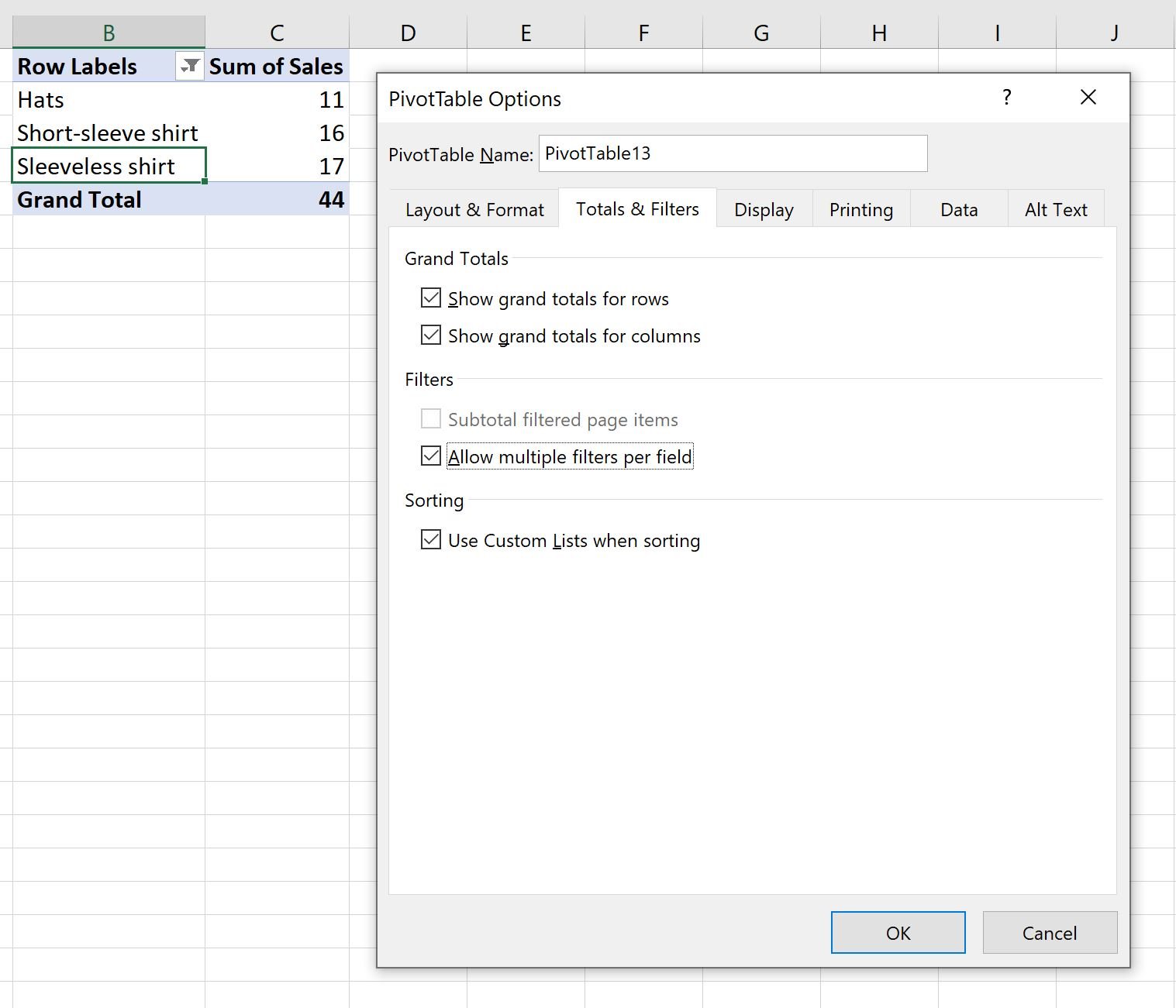
To change this, we can right click on any cell in the pivot table and then click PivotTable Options:

In the new window that appears, click the Totals & Filters tab, then check the box next to Allow multiple filters per field, then click OK:
Now if we filter once again for rows that contain “shirt” then Excel will allow this label filter and the previous value filter to be applied at once:

Notice that we’re able to filter the pivot table to only show rows that contain “shirt” and where the sum of sales is greater than 10.
Additional Resources
The following tutorials explain how to perform other common operations in Excel:
Excel: How to Filter Top 10 Values in Pivot Table
Excel: How to Sort Pivot Table by Grand Total
Excel: How to Calculate the Difference Between Two Pivot Tables