You can use the following syntax to write a nested IFERROR statement in Excel:
=IFERROR(VLOOKUP(G2,A2:B6,2,0),IFERROR(VLOOKUP(G2,D2:E6,2,0), ""))
This particular formula looks for the value in cell G2 in the range A2:B6 and attempts to return the corresponding value in the second column of that range.
If the value in cell G2 is not found in the first range, Excel will then look for it in the range D2:E6 and return the corresponding value in the second column of that range.
If the value in cell G2 is also not found in that range, a blank is returned.
The following example shows how to use this syntax in practice.
Example: Write a Nested IFERROR Statement in Excel
Suppose we have the following datasets in Excel that contain information about various basketball teams:

We can write the following nested IFERROR statement to return the points values associated with various teams:
=IFERROR(VLOOKUP(G2,$A$2:$B$6,2,0),IFERROR(VLOOKUP(G2,$D$2:$E$6,2,0), ""))
The following screenshot shows how to use this formula in practice:
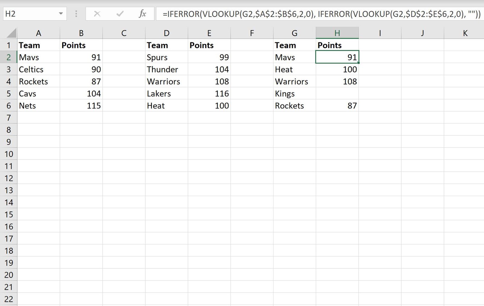
This formula first looks for the team name in column G in the range A2:B6 and attempts to return the corresponding points value.
If the formula doesn’t find the team name in the range A2:B6, it then looks in the range D2:E6 and attempts to return the corresponding points value.
If it doesn’t find the team name in either range, it simply returns a blank value.
We can see that the team name “Kings” doesn’t exist in either range so the points value for that team is simply a blank value.
Note: For this example we created a nested IFERROR statement with two VLOOKUP functions, but we could use however many VLOOKUP functions we’d like depending on how many unique ranges we’re dealing with.
Additional Resources
The following tutorials explain how to perform other common operations in Excel:
How to Compare Two Lists in Excel Using VLOOKUP
How to Use VLOOKUP to Return All Matches in Excel
How to Use VLOOKUP to Return Multiple Columns in Excel