You can use the following syntax to calculate the median value of a filtered range in Excel:
=AGGREGATE(12,1,B2:B13)
The value 12 is a shortcut for calculating the median of a range and the value 1 tells Excel to ignore hidden rows.
The following example shows how to use this function in practice.
Example: Calculate Median of Filtered Rows in Excel
Suppose we have the following dataset that shows the number of sales made during various days by a company:
Next, let’s filter the data to only show the dates that are in January or April.
To do so, highlight the cell range A1:B13. Then click the Data tab along the top ribbon and click the Filter button.
Then click the dropdown arrow next to Date and make sure that only the boxes next to January and April are checked, then click OK:
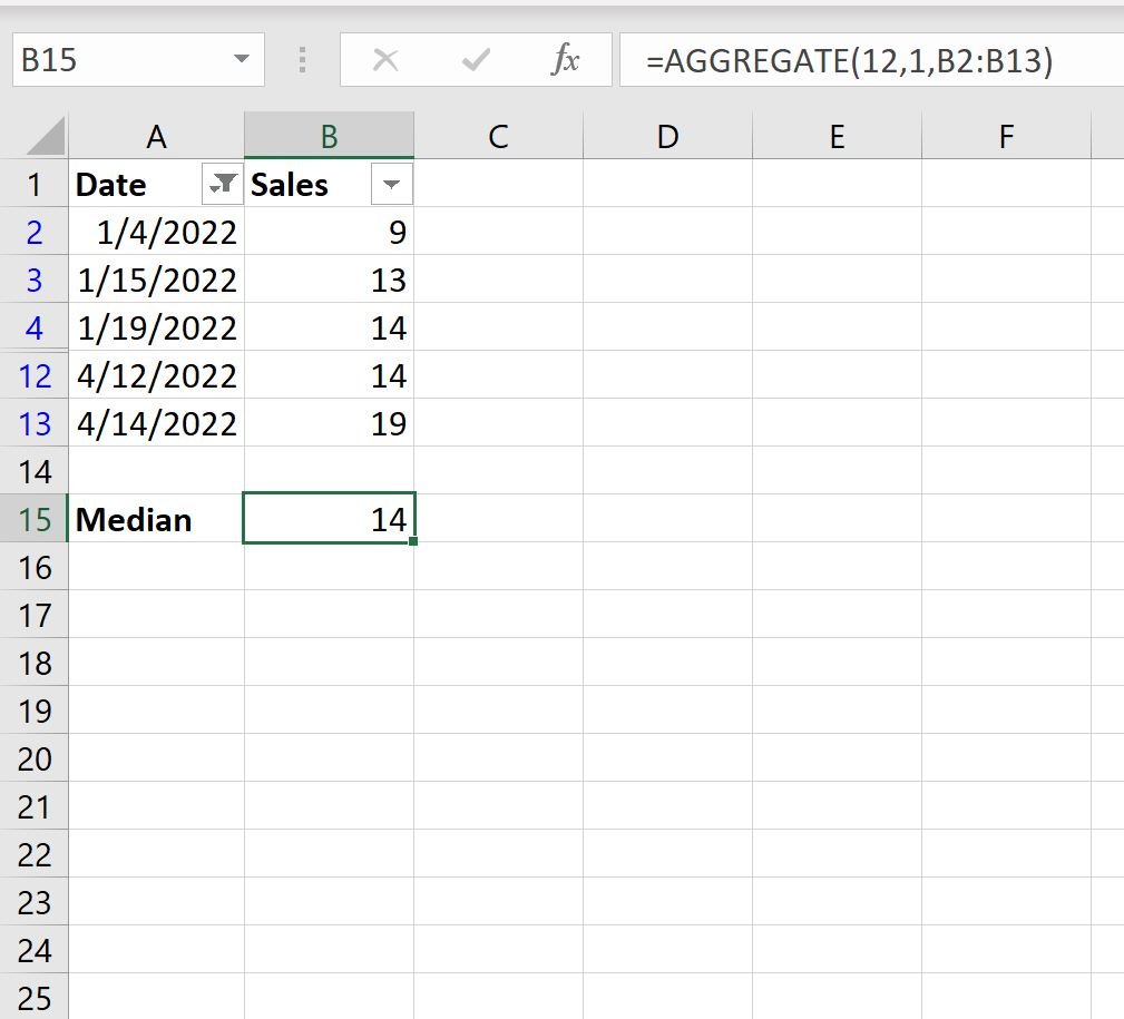
The data will automatically be filtered to only show the rows where the dates are in January or April:
If we attempt to use the MEDIAN() function to find the average value in the Sales column, it will actually return the median of all of the original values:
Instead, we can use the AGGREGATE() function:
This function calculates the median of only the visible rows.
We can manually verify this by calculating the median of the visible rows:
Median of Sales in visible rows: [9, 13, 14, 14, 19]
When the values are arranged in ascending order, the value located in the middle is indeed 14.
Additional Resources
The following tutorials explain how to perform other common operations in Excel:
How to Delete Filtered Rows in Excel
How to Average Filtered Rows in Excel
How to Count Filtered Rows in Excel
How to Sum Filtered Rows in Excel


