The easiest way to filter multiple columns in Excel is to use the Advanced Filter function.
The following examples show how to use this function in two different scenarios:
- Filter for rows that meet multiple conditions
- Filter for rows that meet one of multiple conditions
Example 1: Filter for Rows that Meet Multiple Conditions
Suppose we have the following dataset that shows the total sales of certain products in certain regions for a company:
Now suppose we’d like to filter for rows where the Region is East and the Product is A.
To do so, we can define the following range of cells that contains our criteria:
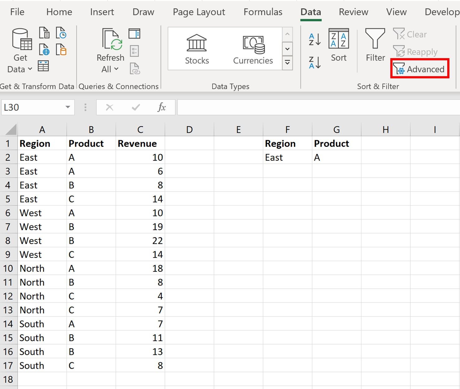
Next, we can click the Data tab and then click the Advanced Filter button:
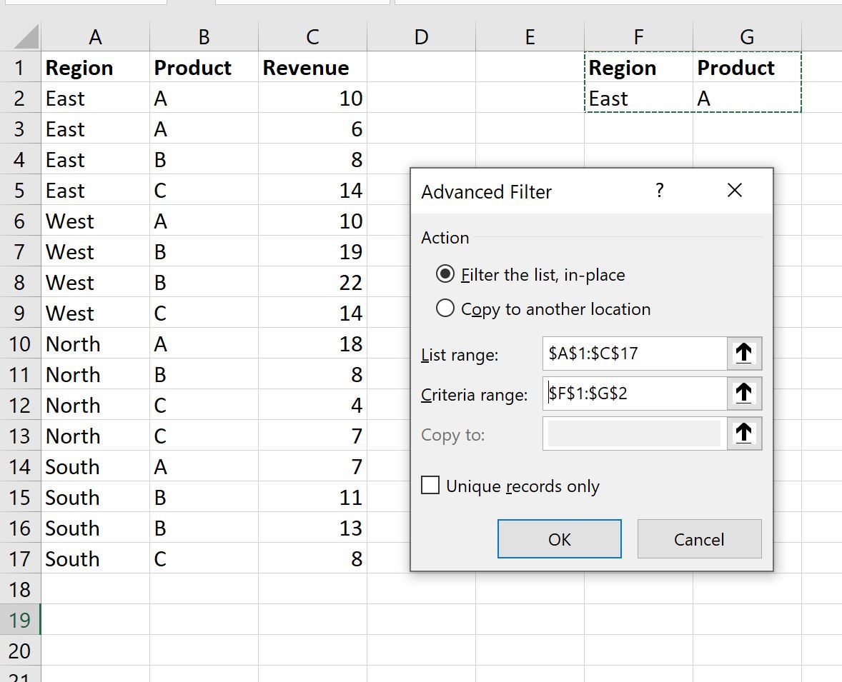
We’ll choose A1:C17 as the list range and F1:G2 as the criteria range:
Once we click OK, the dataset will be filtered to only show rows where the Region is East and the Product is A:
Example 2: Filter for Rows that Meet One of Multiple Conditions
Suppose we have the following dataset that shows the total sales of certain products in certain regions for a company:
Now suppose we’d like to filter for rows where the Region is East or the Product is A.
To do so, we can define the following range of cells that contains our criteria:
Next, we can click the Data tab and then click the Advanced Filter button.
We’ll choose A1:C17 as the list range and F1:G3 as the criteria range:
Once we click OK, the dataset will be filtered to only show rows where the Region is East or the Product is A:
Additional Resources
The following tutorials explain how to perform other common operations in Excel:
How to Sum Filtered Rows in Excel
How to Delete Filtered Rows in Excel


