The following step-by-step example shows how to convert an Excel pivot table to a data table.
Step 1: Enter the Data
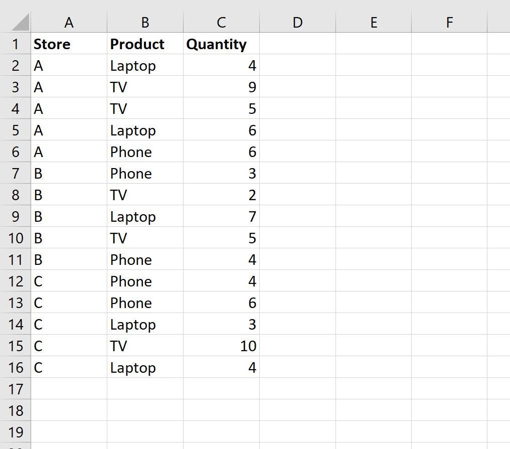
First, let’s enter the following sales data for three different stores:
Step 2: Create the Pivot Table
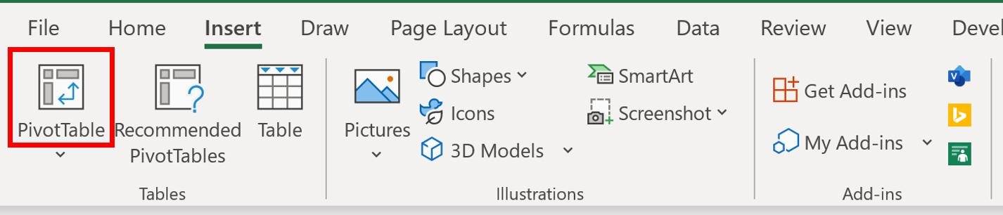
To create a pivot table, click the Insert tab along the top ribbon and then click the PivotTable icon:
In the new window that appears, choose A1:C16 as the range and choose to place the pivot table in cell E1 of the existing worksheet:

Once you click OK, a new PivotTable Fields panel will appear on the right side of the screen.
Drag the Store field to the Rows box, then drag the Product field to the Columns box, then drag the Quantity field to the Values box:

The pivot table will automatically be populated with the following values:

Step 3: Convert Pivot Table to Table
To convert this pivot table to an ordinary data table, simply select the entire pivot table (in this case, we select the range E1:I6) and press Ctrl+C to copy the data.

Then right click the cell where you’d like to paste the data (we’ll choose cell E8) and click the option titled Paste Values:
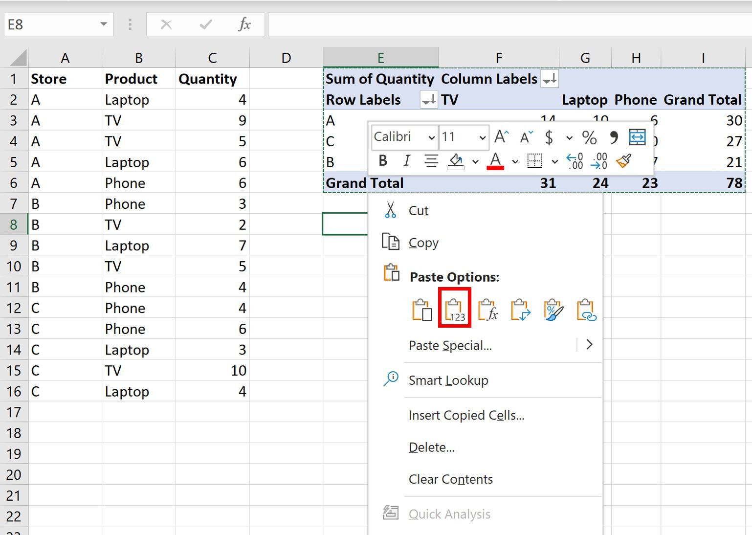
The values from the pivot table will automatically be pasted as regular data values, starting in cell E8:

Notice that this table doesn’t contain any of the fancy formatting or dropdown filters that were in the pivot table.
We’re simply left with a table of regular data values.
Additional Resources
The following tutorials explain how to perform other common tasks in Excel:
How to Create Tables in Excel
How to Group Values in Pivot Table by Range in Excel
How to Group by Month and Year in Pivot Table in Excel