You can use the following formula to calculate the average in Excel only for the cells that contain a specific text:
=AVERAGEIF(A1:A13,"*text*",B1:B13)
This particular formula will calculate the average of the values in the range B1:B13 only for the cells that contain “text” in the range A1:A13.
Note: The asterisks are wildcard characters that tell Excel to ignore any text before or after a specific string.
The following example shows how to use this formula in practice.
Example: Calculate Average If Cell Contains Text
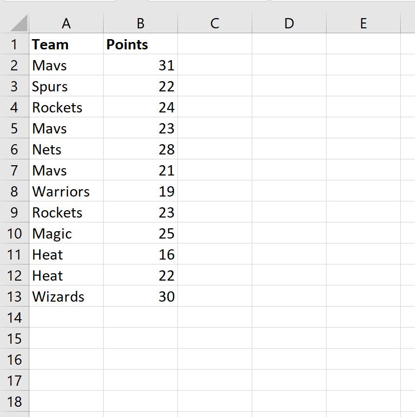
Suppose we have the following dataset that shows the points scored by 12 different basketball players:
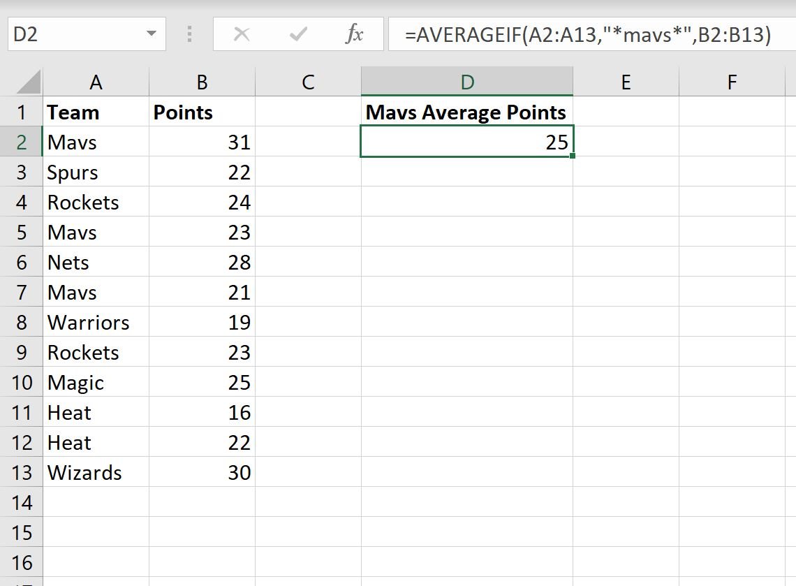
We can use the following formula to calculate the average points scored by players on the “Mavs” team only:
=AVERAGEIF(A2:A13,"*mavs*",B2:B13)
The following screenshot shows how to use this formula in practice:
The average points scored by players on the “Mavs” team is 25.
We can manually verify that this is correct:
Average Points Scored = (31 + 23 + 21) / 3= 25.
Note that this formula is case-insensitive.
That is, we could use “*MAVS*” or “*mavs*” or “*Mavs*” in the formula and Excel will return the same result.
Note: You can find the complete documentation for the AVERAGEIF function here.
Additional Resources
The following tutorials explain how to perform other common tasks in Excel:
How to Calculate Average If Between Two Values in Excel
How to Calculate a Cumulative Average in Excel
How to Find Weighted Moving Averages in Excel


