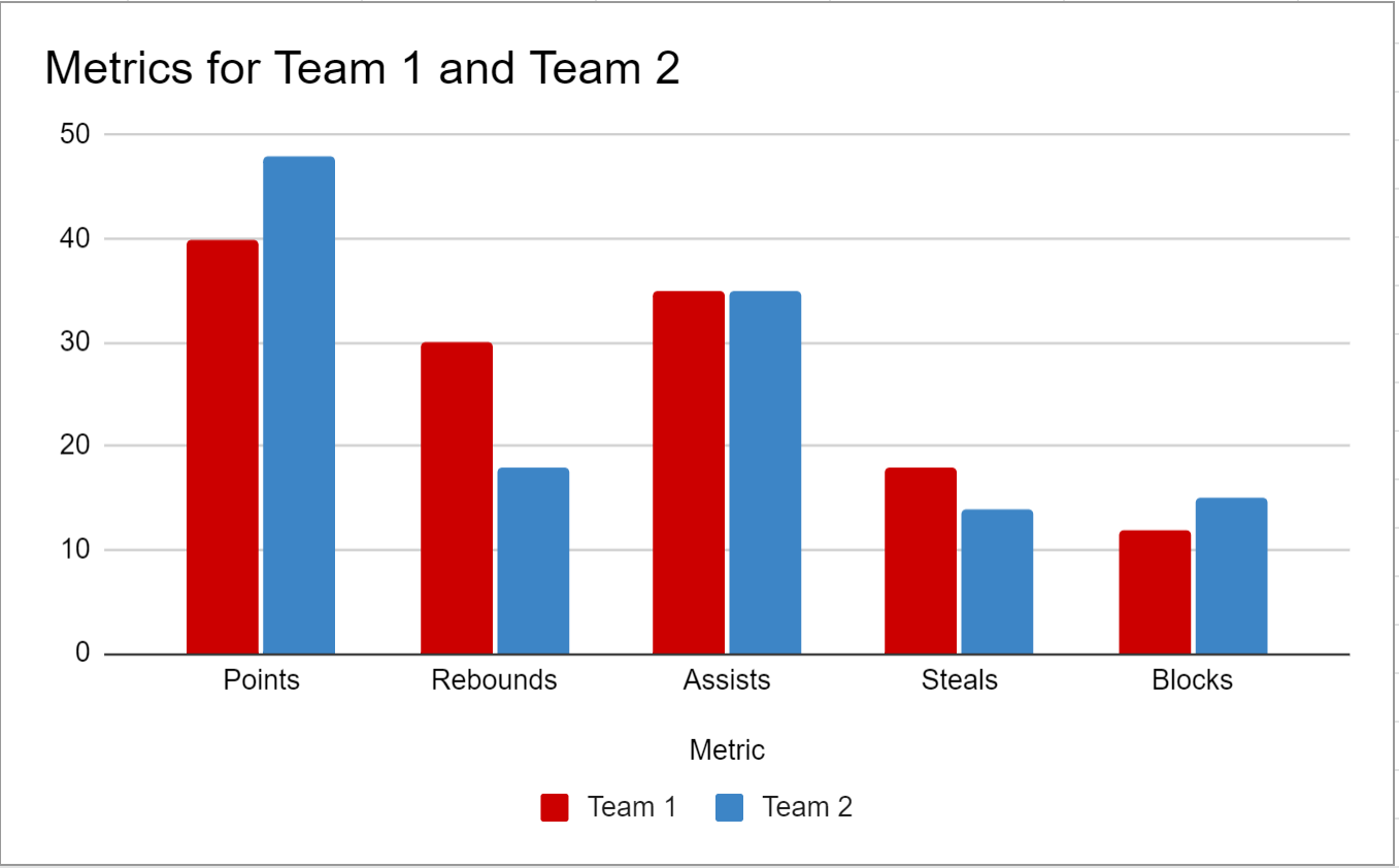
A double bar graph is useful for visualizing two datasets on one graph.
The following step-by-step example shows how to create a double bar graph in Google Sheets.
Step 1: Enter the Data
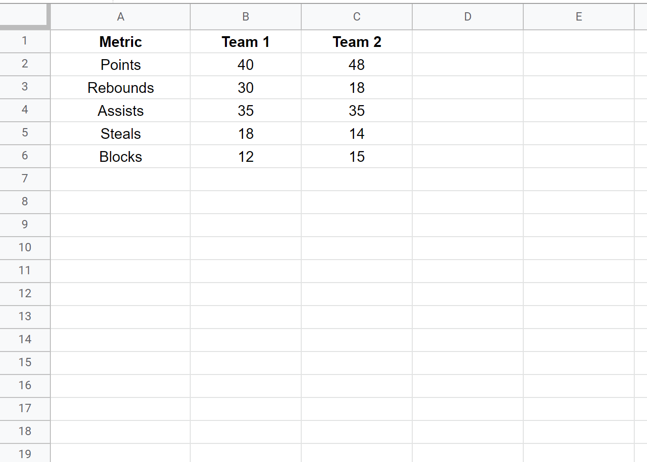
First, let’s enter the values for the following dataset:
Step 2: Create the Double Bar Graph
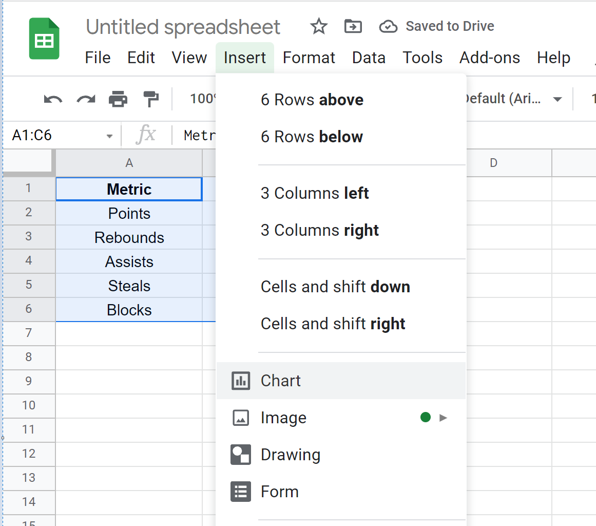
To create a double bar graph for this dataset, we can first highlight the values in the range A1:C6. Then click the Insert tab, then click Chart:
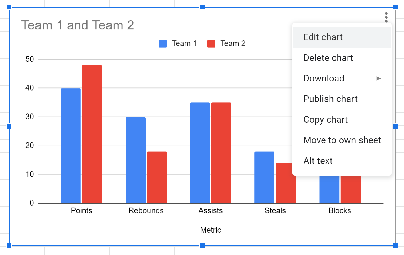
The following double bar graph will appear:
The x-axis displays the various metrics and the y-axis shows the values of those metrics for both Team 1 and Team 2.
Step 3: Customize the Double Bar Graph
To customize the graph, first click anywhere on the graph. Then click the three vertical dots in the top right corner. Then click Edit chart:
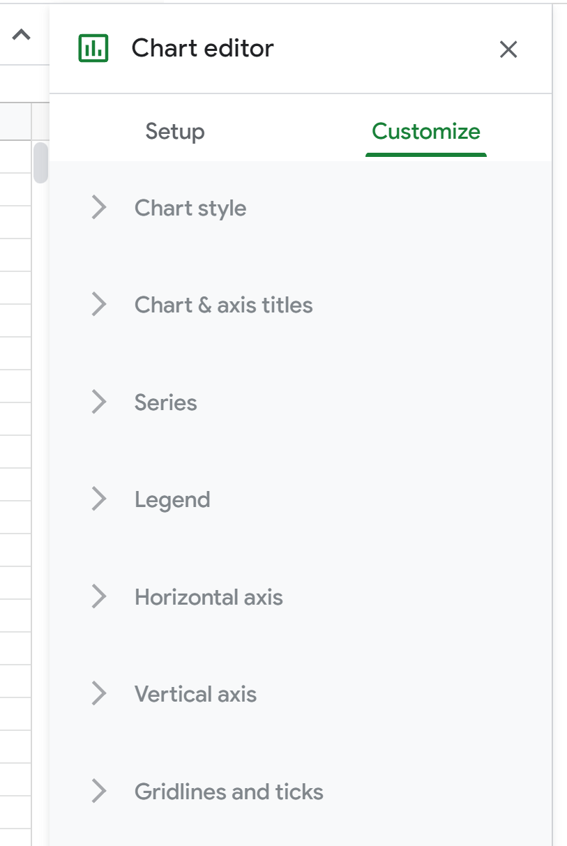
In the Chart editor panel that appears on the right side of the screen, click the Customize tab to see a variety of options for customizing the appearance of the chart:
For example, we can change the chart title, the colors of the bars, and the location of the legend:
Feel free to modify the chart in any way you’d like so that it looks best for your particular situation.
Additional Resources
The following tutorials explain how to create other common charts in Google Sheets:
How to Create a Box Plot in Google Sheets
How to Create a Bubble Chart in Google Sheets
How to Create a Pareto Chart in Google Sheets
How to Create a Pie Chart in Google Sheets


