The normal distribution is the most commonly used distribution in statistics. This tutorial explains how to work with the normal distribution in R using the functions dnorm, pnorm, rnorm, and qnorm.
dnorm
The function dnorm returns the value of the probability density function (pdf) of the normal distribution given a certain random variable x, a population mean μ and population standard deviation σ. The syntax for using dnorm is as follows:
dnorm(x, mean, sd)
The following code illustrates a few examples of dnorm in action:
#find the value of the standard normal distribution pdf at x=0
dnorm(x=0, mean=0, sd=1)
# [1] 0.3989423

#by default, R uses mean=0 and sd=1
dnorm(x=0)
# [1] 0.3989423

#find the value of the normal distribution pdf at x=10 with mean=20 and sd=5
dnorm(x=10, mean=20, sd=5)
# [1] 0.01079819
Typically when you’re trying to solve questions about probability using the normal distribution, you’ll often use pnorm instead of dnorm. One useful application of dnorm, however, is in creating a normal distribution plot in R. The following code illustrates how to do so:
#Create a sequence of 100 equally spaced numbers between -4 and 4
x #create a vector of values that shows the height of the probability distribution
#for each value in x
y #plot x and y as a scatterplot with connected lines (type = "l") and add
#an x-axis with custom labels
plot(x,y, type = "l", lwd = 2, axes = FALSE, xlab = "", ylab = "")
axis(1, at = -3:3, labels = c("-3s", "-2s", "-1s", "mean", "1s", "2s", "3s"))
This generates the following plot:
pnorm
The function pnorm returns the value of the cumulative density function (cdf) of the normal distribution given a certain random variable q, a population mean μ and population standard deviation σ. The syntax for using pnorm is as follows:
pnorm(q, mean, sd)
Put simply, pnorm returns the area to the left of a given value x in the normal distribution. If you’re interested in the area to the right of a given value q, you can simply add the argument lower.tail = FALSE
pnorm(q, mean, sd, lower.tail = FALSE)
The following examples illustrates how to solve some probability questions using pnorm.
Example 1: Suppose the height of males at a certain school is normally distributed with a mean of a standard deviation of
#find percentage of males that are taller than 74 inches in a population with
#mean = 70 and sd = 2
pnorm(74, mean=70, sd=2, lower.tail=FALSE)

# [1] 0.02275013
At this school, 2.275% of males are taller than 74 inches.
Example 2: Suppose the weight of a certain species of otters is normally distributed with a mean of a standard deviation of
#find percentage of otters that weight less than 22 lbs in a population with
#mean = 30 and sd = 5
pnorm(22, mean=30, sd=5)

# [1] 0.05479929
Approximately 5.4799% of this species of otters weigh less than 22 lbs.
Example 3: Suppose the height of plants in a certain region is normally distributed with a mean of a standard deviation of
#find percentage of plants that are less than 14 inches tall, then subtract the
#percentage of plants that are less than 10 inches tall, based on a population
#with mean = 13 and sd = 2
pnorm(14, mean=13, sd=2) - pnorm(10, mean=13, sd=2)

# [1] 0.6246553
Approximately 62.4655% of plants in this region are between 10 and 14 inches tall.
qnorm
The function qnorm returns the value of the inverse cumulative density function (cdf) of the normal distribution given a certain random variable p, a population mean μ and population standard deviation σ. The syntax for using qnorm is as follows:
qnorm(p, mean, sd)
Put simply, you can use qnorm to find out what the Z-score is of the pth quantile of the normal distribution.
The following code illustrates a few examples of qnorm in action:
#find the Z-score of the 99th quantile of the standard normal distribution
qnorm(.99, mean=0, sd=1)
# [1] 2.326348

#by default, R uses mean=0 and sd=1
qnorm(.99)
# [1] 2.326348

#find the Z-score of the 95th quantile of the standard normal distribution
qnorm(.95)
# [1] 1.644854

#find the Z-score of the 10th quantile of the standard normal distribution
qnorm(.10)
# [1] -1.281552
rnorm
The function rnorm generates a vector of normally distributed random variables given a vector length n, a population mean μ and population standard deviation σ. The syntax for using rnorm is as follows:
rnorm(n, mean, sd)
The following code illustrates a few examples of rnorm in action:
#generate a vector of 5 normally distributed random variables with mean=10 and sd=2
five #generate a vector of 1000 normally distributed random variables with mean=50 and sd=5
narrowDistribution #generate a vector of 1000 normally distributed random variables with mean=50 and sd=25
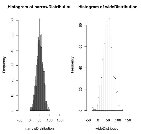
wideDistribution #generate two histograms to view these two distributions side by side, specify
#50 bars in histogram and x-axis limits of -50 to 150
par(mfrow=c(1, 2)) #one row, two columns
hist(narrowDistribution, breaks=50, xlim=c(-50, 150))
hist(wideDistribution, breaks=50, xlim=c(-50, 150))
This generates the following histograms:
Notice how the wide distribution is much more spread out compared to the narrow distribution. This is because we specified the standard deviation in the wide distribution to be 25 compared to just 15 in the narrow distribution. Also notice that both histograms are centered around the mean of 50.


