In statistics, we often want to know how influential different observations are in regression models.
One way to calculate the influence of observations is by using a metric known as DFFITS, which stands for “difference in fits.”
This metric tells us how much the predictions made by a regression model change when we leave out an individual observation.
This tutorial shows a step-by-step example of how to calculate and visualize DFFITS for each observation in a model in R.
Step 1: Build a Regression Model
First, we’ll build a multiple linear regression model using the built-in mtcars dataset in R:
#load the dataset
data(mtcars)

#fit a regression model
model #view model summary
summary(model)

Coefficients:
             Estimate Std. Error t value Pr(>|t|)
(Intercept) 30.735904   1.331566  23.083
Step 2: Calculate DFFITS for each Observation
Next, we’ll use the built-in dffits() function to calculate the DFFITS value for each observation in the model:
#calculate DFFITS for each observation in the model
dffits as.data.frame(dffits(model))

#display DFFITS for each observation
dffits

                    dffits(model)
Mazda RX4             -0.14633456
Mazda RX4 Wag         -0.14633456
Datsun 710            -0.19956440
Hornet 4 Drive         0.11540062
Hornet Sportabout      0.32140303
Valiant               -0.26586716
Duster 360             0.06282342
Merc 240D             -0.03521572
Merc 230              -0.09780612
Merc 280              -0.22680622
Merc 280C             -0.32763355
Merc 450SE            -0.09682952
Merc 450SL            -0.03841129
Merc 450SLC           -0.17618948
Cadillac Fleetwood    -0.15860270
Lincoln Continental   -0.15567627
Chrysler Imperial      0.39098449
Fiat 128               0.60265798
Honda Civic            0.35544919
Toyota Corolla         0.78230167
Toyota Corona         -0.25804885
Dodge Challenger      -0.16674639
AMC Javelin           -0.20965432
Camaro Z28            -0.08062828
Pontiac Firebird       0.67858692
Fiat X1-9              0.05951528
Porsche 914-2          0.09453310
Lotus Europa           0.55650363
Ford Pantera L         0.31169050
Ferrari Dino          -0.29539098
Maserati Bora          0.76464932
Volvo 142E            -0.24266054
Typically we take a closer look at observations that have DFFITS values greater than a threshold of 2√p/n where:
- p: Number of predictor variables used in the model
- n: Number of observations used in the model
In this example, the threshold would be 0.5:
#find number of predictors in model
p length(model$coefficients)-1

#find number of observations
n nrow(mtcars)

#calculate DFFITS threshold value
thresh sqrt(p/n)

thresh

[1] 0.5
We can sort the observations based on their DFFITS values to see if any of them exceed the threshold:
#sort observations by DFFITS, descending
dffits[order(-dffits['dffits(model)']), ]

 [1]  0.78230167  0.76464932  0.67858692  0.60265798  0.55650363  0.39098449
 [7]  0.35544919  0.32140303  0.31169050  0.11540062  0.09453310  0.06282342
[13]  0.05951528 -0.03521572 -0.03841129 -0.08062828 -0.09682952 -0.09780612
[19] -0.14633456 -0.14633456 -0.15567627 -0.15860270 -0.16674639 -0.17618948
[25] -0.19956440 -0.20965432 -0.22680622 -0.24266054 -0.25804885 -0.26586716
[31] -0.29539098 -0.32763355
We can see that the first five observations have a DFFITS value greater than 0.5, which means we may want to investigate these observations closer to determine if they’re highly influential in the model.
Step 3: Visualize the DFFITS for each Observation
Lastly, we can create a quick plot to visualize the DFFITS for each observation:
#plot DFFITS values for each observation
plot(dffits(model), type = 'h')

#add horizontal lines at absolute values for threshold
abline(h = thresh, lty = 2)
abline(h = -thresh, lty = 2)
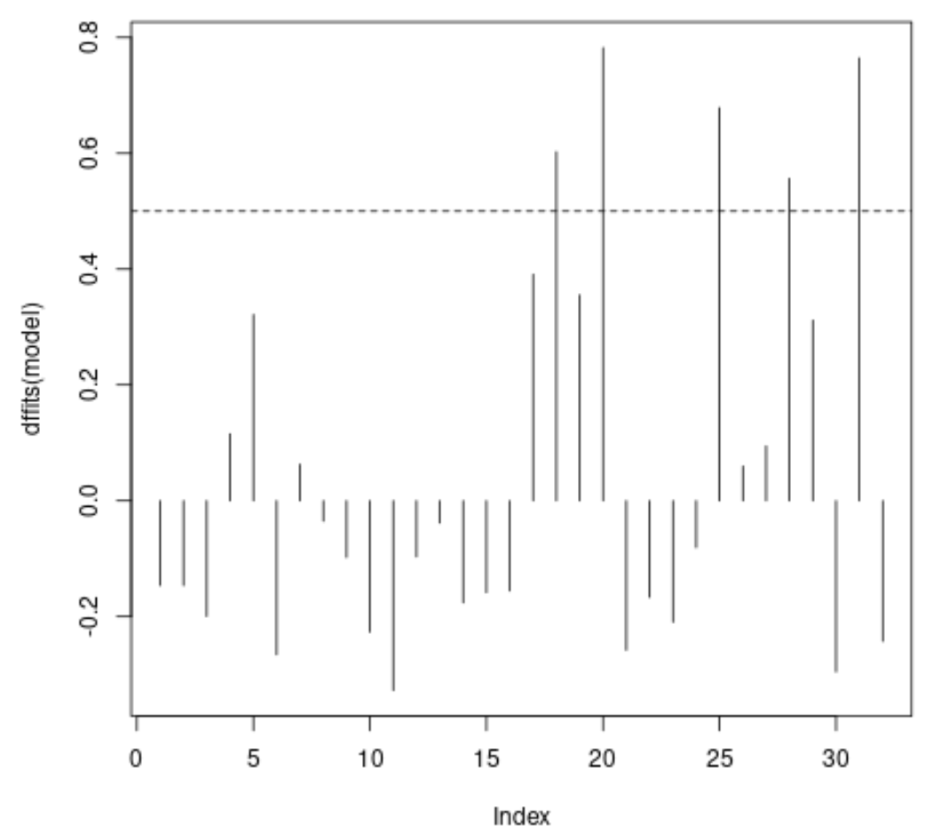
The x-axis displays the index of each observation in the dataset and the y-value displays the corresponding DFFITS value for each observation.
Additional Resources
How to Perform Simple Linear Regression in R
How to Perform Multiple Linear Regression in R
How to Calculate Leverage Statistics in R
How to Create a Residual Plot in R