A continuity correction is applied when you want to use a continuous distribution to approximate a discrete distribution. Typically it is used when you want to use a normal distribution to approximate a binomial distribution.
Recall that the binomial distribution tells us the probability of obtaining x successes in n trials, given the probability of success in a single trial is p. To answer questions about probability with a binomial distribution we could simply use a Binomial Distribution Calculator, but we could also approximate the probability using a normal distribution with a continuity correction.
A continuity correction is the name given to adding or subtracting 0.5 to a discrete x-value.
For example, suppose we would like to find the probability that a coin lands on heads less than or equal to 45 times during 100 flips. That is, we want to find P(X ≤ 45). To use the normal distribution to approximate the binomial distribution, we would instead find P(X ≤ 45.5).
The following table shows when you should add or subtract 0.5, based on the type of probability you’re trying to find:
| Using Binomial Distribution | Using Normal Distribution with Continuity Correction |
|---|---|
| X = 45 | 44.5 |
| X ≤ 45 | X |
| X | X |
| X ≥ 45 | X > 44.5 |
| X > 45 | X > 45.5 |
Note:
It’s only appropriate to apply a continuity correction to the normal distribution to approximate the binomial distribution when n*p and n*(1-p) are both at least 5.
For example, suppose n = 15 and p = 0.6. In this case:
n*p = 15 * 0.6 = 9
n*(1-p) = 15 * (1 – 0.6) = 15 * (0.4) = 6
Since both of these numbers are greater than or equal to 5, it would be okay to apply a continuity correction in this scenario.
The following example illustrates how to apply a continuity correction to the normal distribution to approximate the binomial distribution.
Example of Applying a Continuity Correction
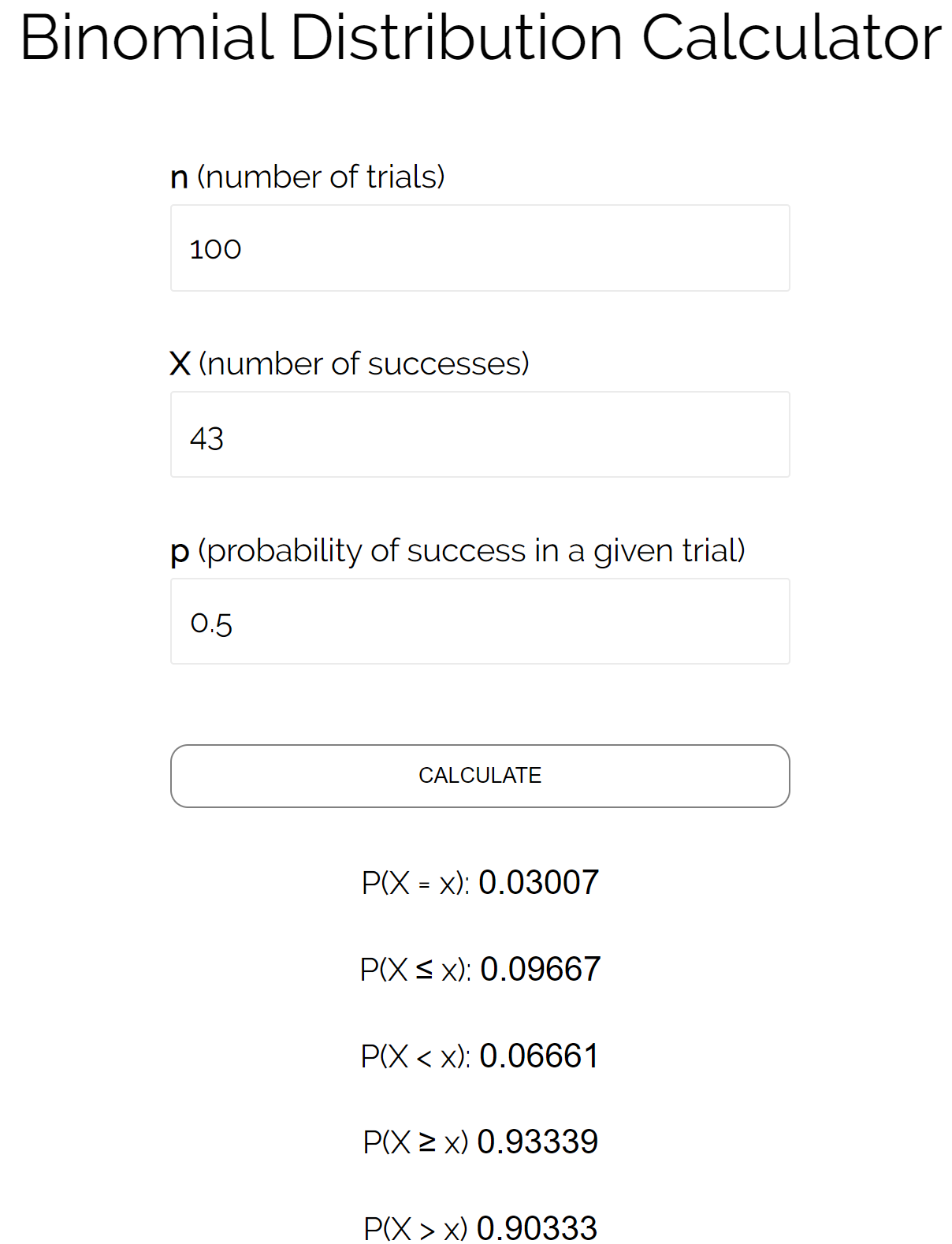
Suppose we want to know the probability that a coin lands on heads less than or equal to 43 times during 100 flips. In this case:
n = number of trials = 100
X = number of successes = 43
p = probability of success in a given trial = 0.50
We can plug these numbers into the Binomial Distribution Calculator to see that the probability of the coin landing on heads less than or equal to 43 times is 0.09667.
To approximate the binomial distribution by applying a continuity correction to the normal distribution, we can use the following steps:
Step 1: Verify that n*p and n*(1-p) are both at least 5.
n*p = 100*0.5 = 50
n*(1-p) = 100*(1 – 0.5) = 100*0.5 = 50
Both numbers are greater than or equal to 5, so we’re good to proceed.
Step 2: Determine if you should add or subtract 0.5
Referring to the table above, we see that we’re supposed to add 0.5 when we’re working with a probability in the form of X ≤ 43. Thus, we will be finding P(X
Step 3: Find the mean (μ) and standard deviation (σ) of the binomial distribution.
μ = n*p = 100*0.5 = 50
σ = √n*p*(1-p) = √100*.5*(1-.5) = √25 = 5
Step 4: Find the z-score using the mean and standard deviation found in the previous step.
z = (x – μ) / σ = (43.5 – 50) / 5 = -6.5 / 5 = -1.3.
Step 5: Use the Z table to find the probability associated with the z-score.
According to the Z table, the probability associated with z = -1.3 is 0.0968.
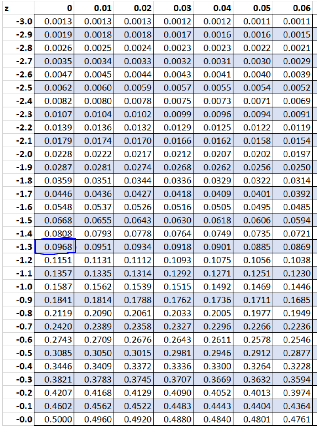
Thus, the exact probability we found using the binomial distribution was 0.09667 while the approximate probability we found using the continuity correction with the normal distribution was 0.0968. These two values are pretty close.
When to Use a Continuity Correction
Before modern statistical software existed and calculations had to be done manually, continuity corrections were often used to find probabilities involving discrete distributions. Today, continuity corrections play less of a role in computing probabilities since we can typically rely on software or calculators to calculate probabilities for us.
Instead, it’s simply a topic discussed in statistics classes to illustrate the relationship between a binomial distribution and a normal distribution and to show that it’s possible for a normal distribution to approximate a binomial distribution by applying a continuity correction.
Continuity Correction Calculator
Use the Continuity Correction Calculator to automatically apply a continuity correction to a normal distribution to approximate binomial probabilities.