A contingency table (sometimes called “crosstabs”) is a type of table that summarizes the relationship between two categorical variables.
Fortunately it’s easy to create a contingency table for variables in Excel by using the pivot table function. This tutorial shows an example of how to do so.
Example: Contingency Table in Excel
Suppose we have the following dataset that shows information for 20 different product orders, including the type of product purchased (TV, computer, or radio) along with the country (A, B, or C) that the product was purchased in:

Use the following steps to create a contingency table for this dataset:
Step 1: Select the PivotTable option.
Click the Insert tab, then click PivotTable.

In the window that pops up, choose A1:C21 for the range of values. Then choose a location to place the pivot table in. We’ll choose cell E2 within the existing worksheet:

Once you click OK, an empty contingency table will appear in cell E2.

Step 2: Populate the contingency table.
In the window that appears on the right, drag Country into the box titled Rows, drag Product into the box titled Columns, and drag Order Number into the box titled Values:

Note: If Values first appears as “Sum of Order Number” simply click the dropdown arrow and select Value Field Settings. Then choose Count and click OK.
Once you do so, the frequency values will automatically be populated in the contingency table:
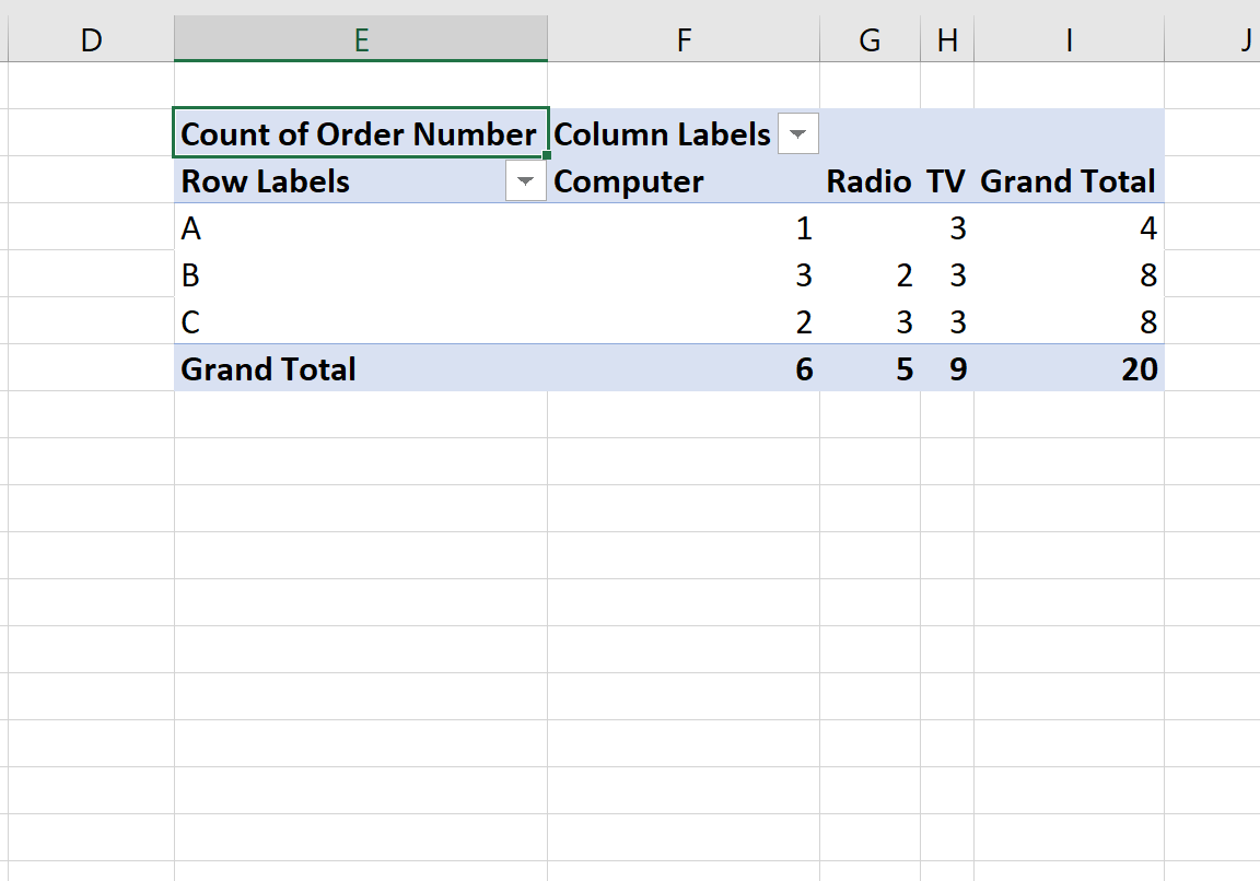
Step 3: Interpret the contingency table.
The way to interpret the values in the table is as follows:
Row Totals:
- A total of 4 orders were made from country A.
- A total of 8 orders were made from country B.
- A total of 8 orders were made from country C.
Column Totals:
- A total of 6 computers were purchased.
- A total of 5 radios were purchased.
- A total of 9 TV’s were purchased.
Individual Cells:
- A total of 1 computer was purchased from country A.
- A total of 3 computers were purchased from country B.
- A total of 2 computers were purchased from country C.
- A total of 0 radios were purchased from country A.
- A total of 2 radios were purchased from country B.
- A total of 3 radios were purchased from country C.
- A total of 3 TV’s were purchased from country A.
- A total of 3 TV’s were purchased from country B.
- A total of 3 TV’s were purchased from country C.
Additional Resources
How to Create a Contingency Table in R
How to Create a Contingency Table in Python