In statistics, we often take samples from a population and use the data from the sample to draw conclusions about the population as a whole.
One commonly used sampling method is cluster sampling, in which a population is split into clusters and all members of some clusters are chosen to be included in the sample.
The following step-by-step example shows how to perform cluster sampling in Excel.
Step 1: Enter the Data
First, let’s enter the following dataset into Excel:
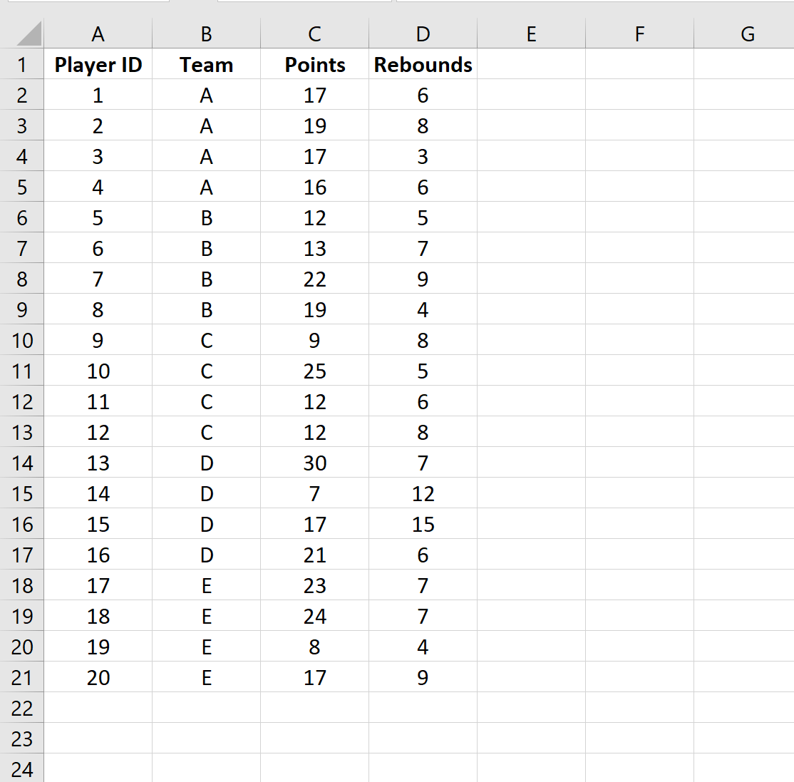
Next, we’ll perform cluster sampling in which we randomly select two teams and choose to include every player from those two teams in the final sample.
Step 2: Find Unique Values
Next, type in =UNIQUE(B2:B21) to produce an array of unique values from the Team column:

Next, we’ll type an integer (starting at 1) next to each unique team name:

Step 3: Select Random Clusters
Next, we’ll type =RANDBETWEEN(G2, G6) to randomly select one of the integers from the list:
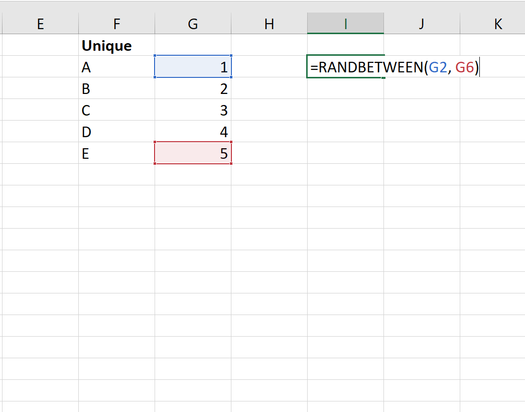
Once we click ENTER, we can see that the value 5 was randomly selected. The team associated with this value is team E, which represents the first team we’ll include in our final sample.

Next, double click any cell and press Enter. A new number will be selected from the =RANDBETWEEN(G2, G6) function.

We can see that the value 3 was randomly selected. The team associated with this value is team C, which represents the second team we’ll include in our final sample.
Step 4: Filter the Final Sample
The final sample will simply include all players who belong to either team C or team E.
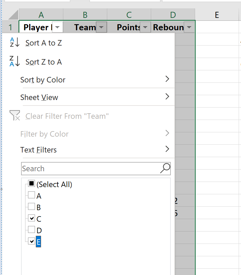
To filter for just these players, highlight all of the data. Then click the Data tab along the top ribbon and then click the Filter button within the Sort & Filter group.
When the filter appears above each column, click the dropdown arrow next to the Team column and check the boxes next to teams C and E only:
Once you click OK, the dataset will be filtered to only show players on team C or team E:

This represents our final sample.
Our cluster sampling is complete because we randomly chose two teams and included each player from those two teams in our final sample.
Additional Resources
The following tutorials explain how to select other types of samples from a population using Excel:
How to Select a Random Sample in Excel
How to Perform Systematic Sampling in Excel
How to Perform Stratified Sampling in Excel