The binomial distribution describes the probability of obtaining k successes in n binomial experiments.
If a random variable X follows a binomial distribution, then the probability that X = k successes can be found by the following formula:
P(X=k) = nCk * pk * (1-p)n-k
where:
- n: number of trials
- k: number of successes
- p: probability of success on a given trial
- nCk: the number of ways to obtain k successes in n trials
The binomial probability distribution tends to be bell-shaped when one or more of the following two conditions occur:
1. The sample size (n) is large.
2. The probability of success on a given trial (p) is close to 0.5.
However, the binomial probability distribution tends to be skewed when neither of these conditions occur. To illustrate this, consider the following examples:
Example 1: Sample Size (n) is Large
The following chart displays the probability distribution for when n = 200 and p = 0.5.
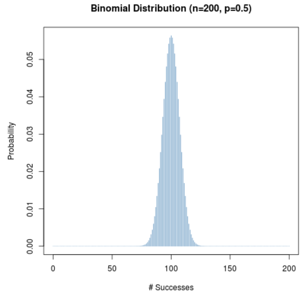
The x-axis displays the number of successes during 200 trials and the y-axis displays the probability of that number of successes occurring.
Since both (1) the sample size is large and (2) the probability of success on a given trial is close to 0.5, the probability distribution is bell-shaped.
Even when the probability of success on a given trial (p) is not close to 0.5, the probability distribution will still be bell-shaped as long as the sample size (n) is large. To illustrate this, consider the following two scenarios when p = 0.2 and p = 0.8.
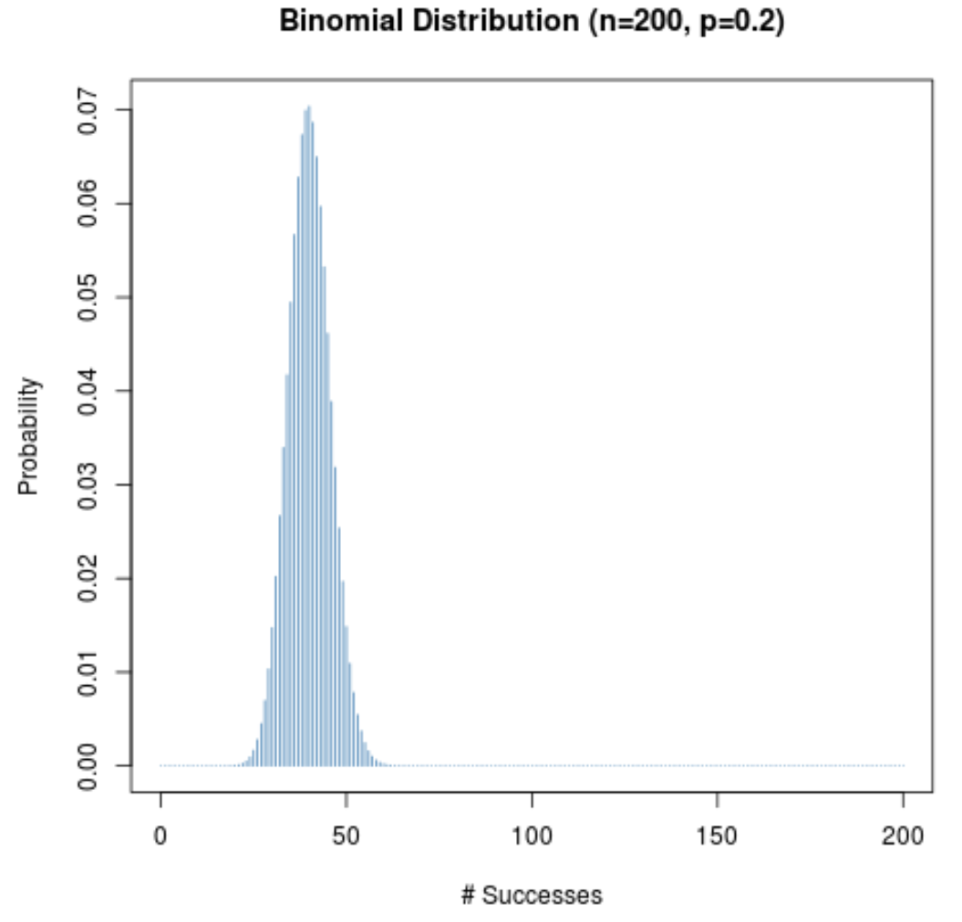
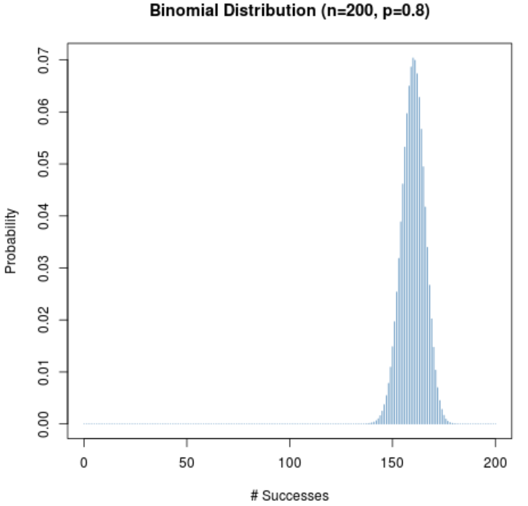
Notice how the probability distribution is bell-shaped in both scenarios.
Example 2: Probability of Success (p) is Close to 0.5
The following chart displays the probability distribution for when n = 10 and p = 0.4.
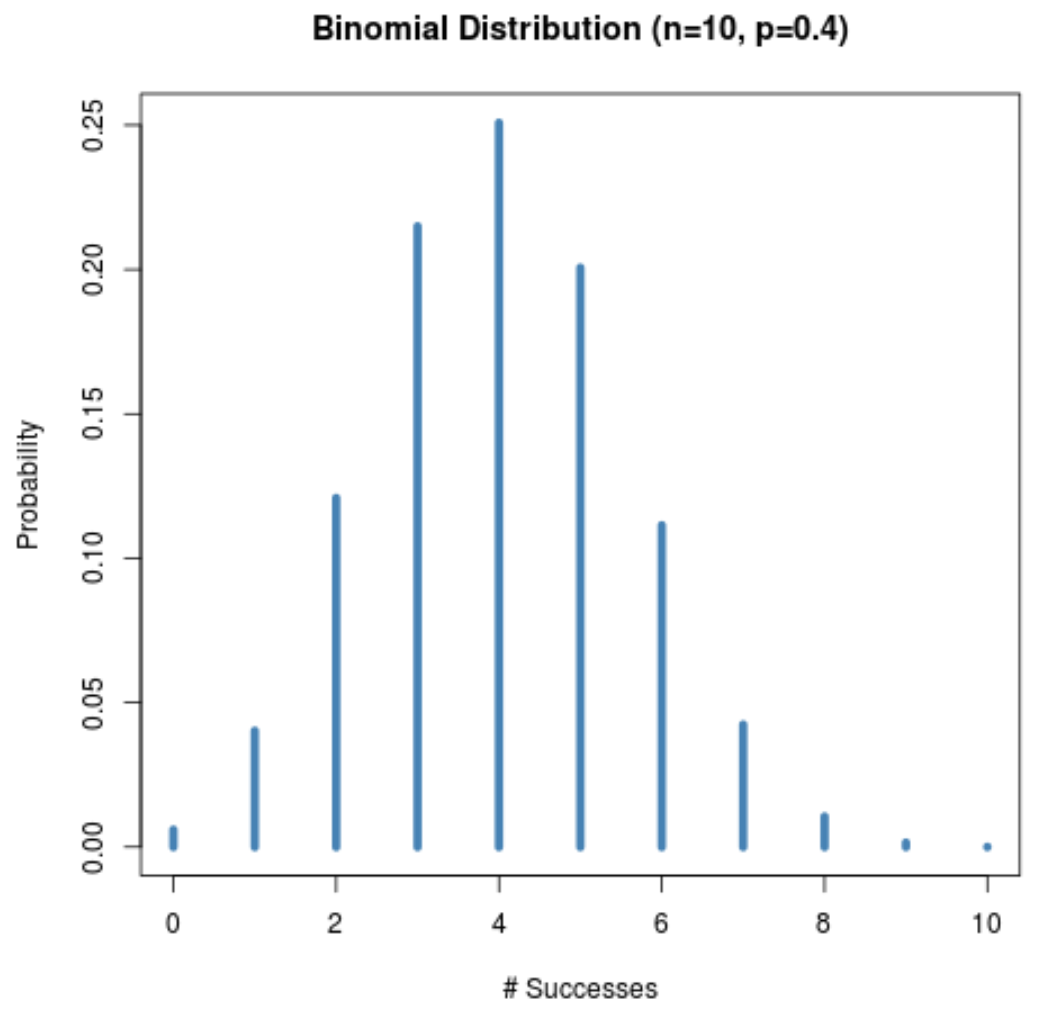
Although the sample size (n = 10) is small, the probability distribution is still bell-shaped because the probability of success on a given trial (p = 0.4) is close to 0.5
Example 3: Skewed Binomial Distributions
When neither (1) the sample size is large nor (2) the probability of success on a given trial is close to 0.5, the binomial probability distribution will be skewed to the left or right.
For example, the following plot shows the probability distribution when n = 20 and p = 0.1.
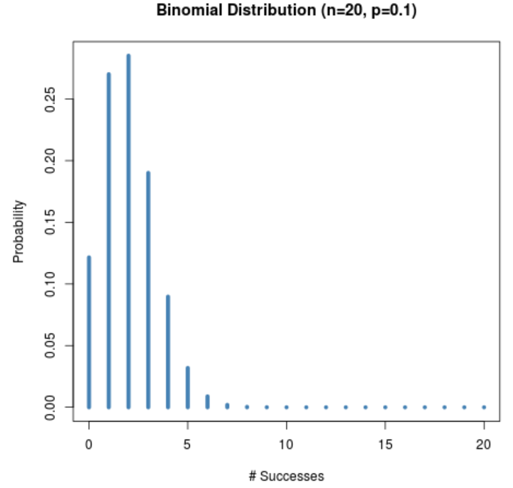
Notice how the distribution is skewed to the right.
And the following plot shows the probability distribution when n = 20 and p = 0.9.
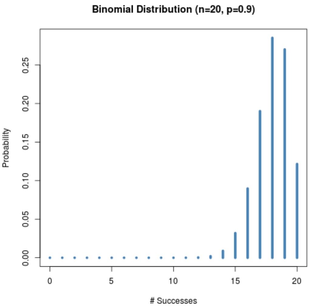
Notice how the distribution is skewed to the left.
Ending Notes
Each of the charts in this post were created using the statistical programming language R. Learn how to plot your own binomial probability distributions in R using this tutorial.