In statistics, we use hypothesis tests to determine if some assumption about a population parameter is true.
A hypothesis test always has the following two hypotheses:
Null hypothesis (H0): The sample data is consistent with the prevailing belief about the population parameter.
Alternative hypothesis (HA): The sample data suggests that the assumption made in the null hypothesis is not true. In other words, there is some non-random cause influencing the data.
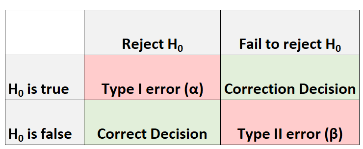
Whenever we conduct a hypothesis test, there are always four possible outcomes:
There are two types of errors we can commit:
- Type I Error: We reject the null hypothesis when it is actually true. The probability of committing this type of error is denoted as α.
- Type II Error: We fail to reject the null hypothesis when it is actually false. The probability of committing this type of error is denoted as β.
The Relationship Between Alpha and Beta
Ideally researchers want both the probability of committing a type I error and the probability of committing a type II error to be low.
However, a tradeoff exists between these two probabilities. If we decrease the alpha level, we can decrease the probability of rejecting a null hypothesis when it’s actually true, but this actually increases the beta level – the probability that we fail to reject the null hypothesis when it actually is false.
The Relationship Between Power and Beta
The power of a hypothesis test refers to the probability of detecting an effect or difference when an effect or difference is actually present. In other words, it’s the probability of correctly rejecting a false null hypothesis.
It is calculated as:
Power = 1 – β
In general, researchers want the power of a test to be high so that if some effect or difference does exist, the test is able to detect it.
From the equation above, we can see that the best way to raise the power of a test is to reduce the beta level. And the best way to reduce the beta level is typically to increase the sample size.
The following examples shows how to calculate the beta level of a hypothesis test and demonstrate why increasing the sample size can lower the beta level.
Example 1: Calculate Beta for a Hypothesis Test
Suppose a researcher wants to test if the mean weight of widgets produced at a factory is less than 500 ounces. It is known that the standard deviation of the weights is 24 ounces and the researcher decides to collect a random sample of 40 widgets.
He will perform the following hypothesis at α = 0.05:
- H0: μ = 500
- HA: μ
Now imagine that the mean weight of widgets being produced is actually 490 ounces. In other words, the null hypothesis should be rejected.
We can use the following steps to calculate the beta level – the probability of failing to reject the null hypothesis when it actually should be rejected:
Step 1: Find the non-rejection region.
According to the Critical Z Value Calculator, the left-tailed critical value at α = 0.05 is -1.645.
Step 2: Find the minimum sample mean we will fail to reject.
The test statistic is calculated as z = (x – μ) / (s/√n)
Thus, we can solve this equation for the sample mean:
- x = μ – z*(s/√n)
- x = 500 – 1.645*(24/√40)
- x = 493.758
Step 3: Find the probability of the minimum sample mean actually occurring.
We can calculate this probability as:
- P(Z ≥ (493.758 – 490) / (24/√40))
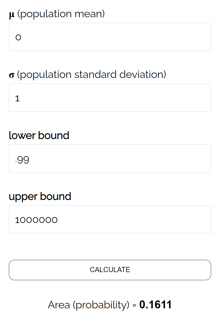
- P(Z ≥ 0.99)
According to the Normal CDF Calculator, the probability that Z ≥ 0.99 is 0.1611.
Thus, the beta level for this test is β = 0.1611. This means there is a 16.11% chance of failing to detect the difference if the real mean is 490 ounces.
Example 2: Calculate Beta for a Test with a Larger Sample Size
Now suppose the researcher performs the exact same hypothesis test but instead uses a sample size of n = 100 widgets. We can repeat the same three steps to calculate the beta level for this test:
Step 1: Find the non-rejection region.
According to the Critical Z Value Calculator, the left-tailed critical value at α = 0.05 is -1.645.
Step 2: Find the minimum sample mean we will fail to reject.
The test statistic is calculated as z = (x – μ) / (s/√n)
Thus, we can solve this equation for the sample mean:
- x = μ – z*(s/√n)
- x = 500 – 1.645*(24/√100)
- x = 496.05
Step 3: Find the probability of the minimum sample mean actually occurring.
We can calculate this probability as:
- P(Z ≥ (496.05 – 490) / (24/√100))
- P(Z ≥ 2.52)
According to the Normal CDF Calculator, the probability that Z ≥ 2.52 is 0.0059.
Thus, the beta level for this test is β = 0.0059. This means there is only a .59% chance of failing to detect the difference if the real mean is 490 ounces.
Notice that by simply increasing the sample size from 40 to 100, the researcher was able to reduce the beta level from 0.1611 all the way down to .0059.
Bonus: Use this Type II Error Calculator to automatically calculate the beta level of a test.
Additional Resources
Introduction to Hypothesis Testing
How to Write a Null Hypothesis (5 Examples)
An Explanation of P-Values and Statistical Significance


