You can use the following syntax with the VLOOKUP function in Google Sheets to look up a value in a range and return the corresponding values from multiple columns:
=ArrayFormula(VLOOKUP(A14, A2:D11, {2, 4}, FALSE))
This particular formula looks up the value in cell A14 in the range A2:D11 and returns the corresponding values in columns 2 and 4 of the range.
Note: The FALSE argument tells Google Sheets to look for exact matches instead of approximate matches.
The following example shows how to use this syntax in practice.
Example: Use VLOOKUP to Return Multiple Columns
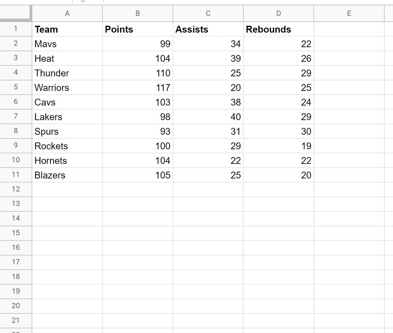
Suppose we have the following dataset in Google Sheets that shows information about various basketball teams:
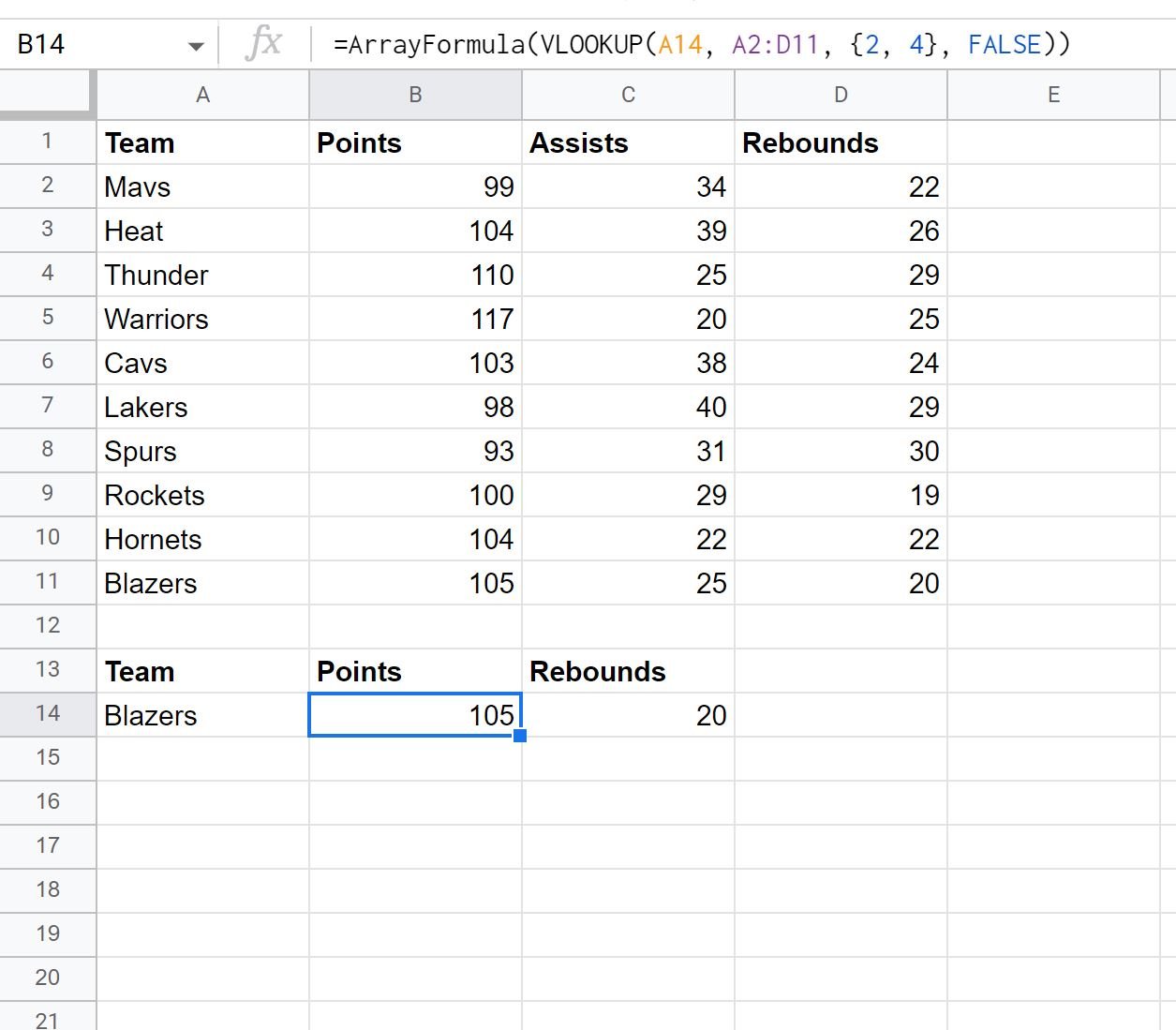
We can use the following formula with VLOOKUP to look up the team “Blazers” in column A and return the corresponding values for points and rebounds:
=ArrayFormula(VLOOKUP(A14, A2:D11, {2, 4}, FALSE))
The following screenshot shows how to use this formula in practice:
The VLOOKUP formula returns the values in the points and rebounds columns for the row where the team contains “Blazers” in the name.
Note that if we change the team name in cell A14, the formula will automatically find the points and rebounds values for the new team.
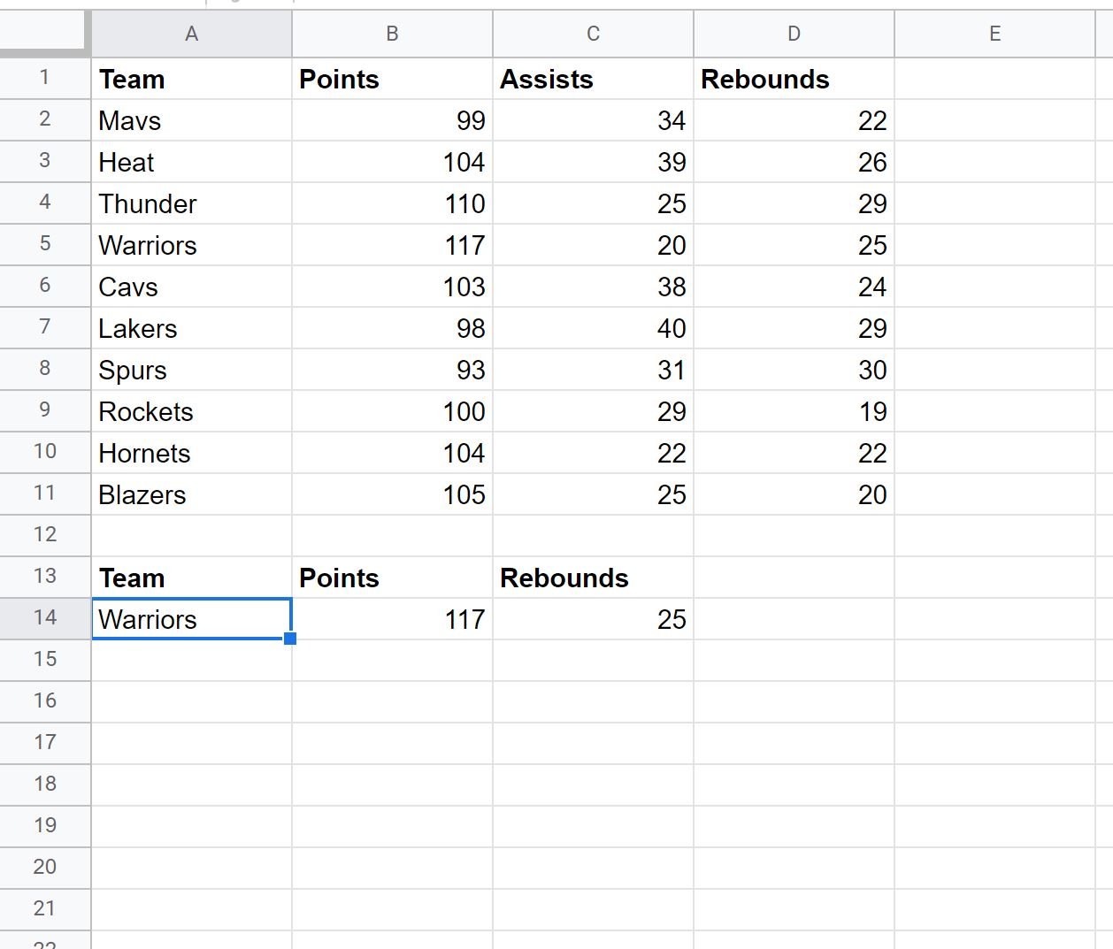
For example, suppose we change the team name to Warriors:
The VLOOKUP formula now returns the values in the points and rebounds columns for the row where the team contains “Warriors” in the name.
Additional Resources
The following tutorials explain how to perform other common tasks in Google Sheets:
Google Sheets: How to Use VLOOKUP From Another Workbook
Google Sheets: Use VLOOKUP to Return All Matches
Google Sheets: Use VLOOKUP with Multiple Criteria


