The Poisson distribution and the normal distribution are two of the most commonly used probability distributions in statistics.
This tutorial provides a quick explanation of each distribution along with two key differences between the distributions.
An Overview: The Poisson Distribution
The Poisson distribution describes the probability of obtaining k successes during a given time interval.
If a random variable X follows a Poisson distribution, then the probability that X = k successes can be found by the following formula:
P(X=k) = λk * e– λ / k!
where:
- λ: mean number of successes that occur during a specific interval
- k: number of successes
- e: a constant equal to approximately 2.71828
For example, suppose a particular hospital experiences an average of 2 births per hour. We can use the formula above to determine the probability of experiencing 3 births in a given hour:
P(X=3) = 23 * e– 2 / 3! = 0.1805
The probability of experiencing 3 births in a given hour is 0.1805.
An Overview: The Normal Distribution
The normal distribution describes the probability that a random variable takes on a value within a given interval.
The probability density function of a normal distribution can be written as:
P(X=x) = (1/σ√2π)e-1/2((x-μ)/σ)2
where:
- σ: Standard deviation of the distribution
- μ: Mean of the distribution
- x: Value for the random variable
For example, suppose the weight of a certain species of otters is normally distributed with μ = 40 pounds and σ = 5 pounds.
If we randomly select an otter from this population, we can use the following formula to find the probability that it weighs between 38 and 42 pounds:
P(38 2π)e-1/2((42-40)/5)2 – (1/σ√2π)e-1/2((38-40)/5)2 = 0.3108
The probability that the randomly selected otter weighs between 38 and 42 pounds is 0.3108.
Difference #1: Discrete vs. Continuous Data
The first difference between the Poisson and normal distribution is the type of data that each probability distribution models.
A Poisson distribution is used when you’re working with discrete data that can only take on integer values equal to or greater than zero. Some examples include:
- Number of calls received per hour at a call center
- Number of customers per day at a restaurant
- Number of car accidents per month
In each scenario, the random variable can only take on a value of 0, 1, 2, 3, etc.
A normal distribution is used when you’re working with continuous data that can take on any value from negative infinity to positive infinity. Some examples include:
- Weight of a certain animal
- Height of a certain plant
- Marathon times of females
- Temperature in Celsius
In these scenarios, the random variables can take on any value like -11.3, 21.343435, 85, etc.
Difference #2: Shape of the Distributions
The second difference between the Poisson and normal distribution is the shape of the distributions.
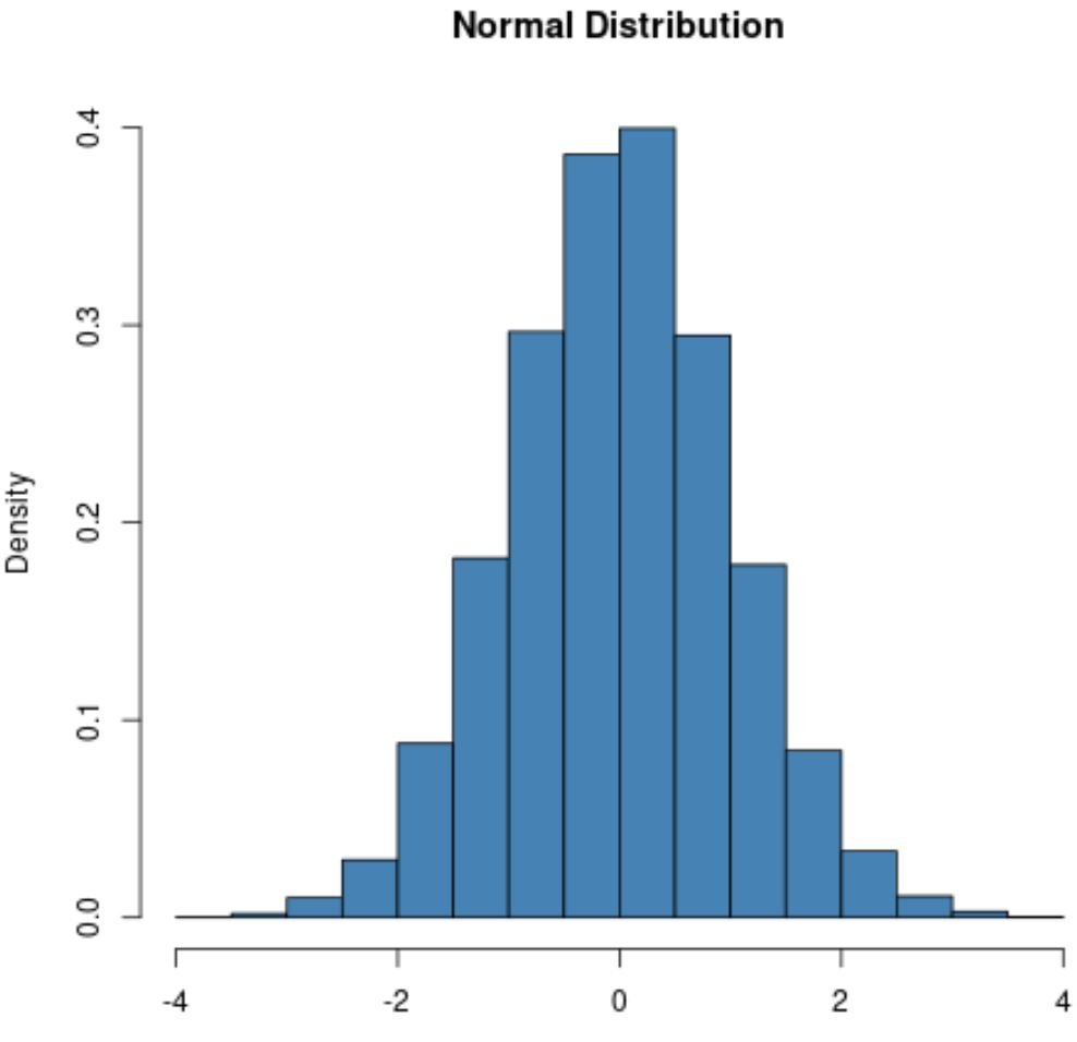
A normal distribution will always exhibit a bell shape:
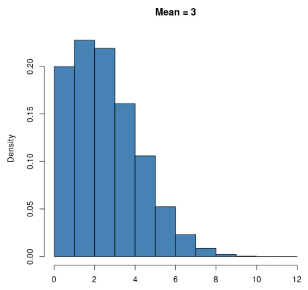
However, the shape of the Poisson distribution will vary based on the mean value of the distribution.
For example, a Poisson distribution with a small value for the mean like μ = 3 will be highly right skewed:
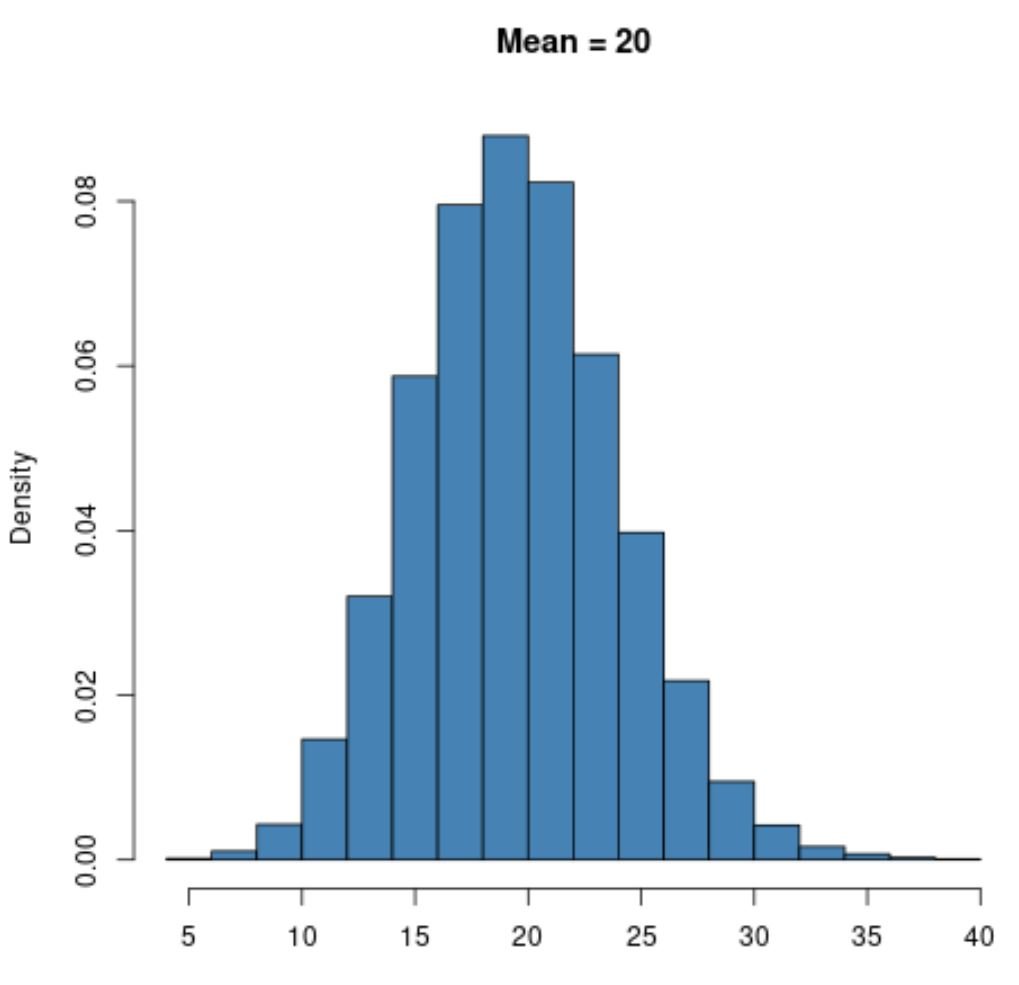
However, a Poisson distribution with a larger value for the mean like μ = 20 will exhibit a bell shape just like the normal distribution:
Notice that the lower bound for a Poisson distribution will always be zero no matter what the value for the mean is because a Poisson distribution can only be used with integer values that are equal to or greater than zero.
Additional Resources
The following tutorials provide additional information about the Poisson distribution:
An Introduction to the Poisson Distribution
The Four Assumptions of the Poisson Distribution
5 Real-Life Examples of the Poisson Distribution
The following tutorials provide additional information about the normal distribution:
An Introduction to the Normal Distribution
6 Real-Life Examples of the Normal Distribution
Normal Distribution Dataset Generator


