How to Perform Piecewise Regression in R (Step-by-Step)

Piecewise regression is a regression method we often use when there are clear “breakpoints” in a dataset.

The following step-by-step example shows how to perform piecewise regression in R.

Step 1: Create the Data

First, let’s create the following data frame:

#view DataFrame
df frame(x=c(1, 2, 3, 4, 5, 6, 7, 8, 9, 10, 11, 12, 13, 14, 15, 16),
                 y=c(2, 4, 5, 6, 8, 10, 12, 13, 15, 19, 24, 28, 31, 34, 39, 44))

#view first six rows of data frame
head(df)

  x  y
1 1  2
2 2  4
3 3  5
4 4  6
5 5  8
6 6 10

Step 2: Visualize the Data

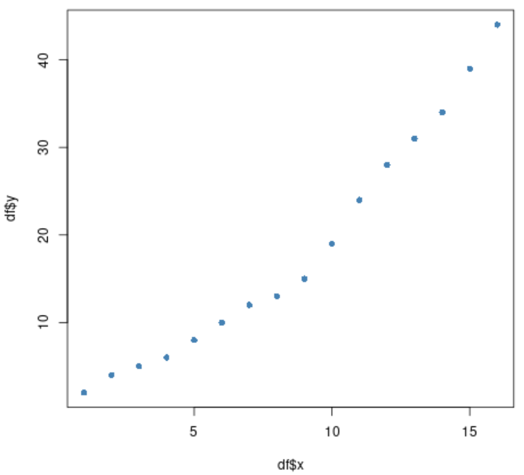
Next, let’s create a scatterplot to visualize the data:

#create scatterplot of x vs. y
plot(df$x, df$y, pch=16, col='steelblue')

We can see that the relationship between x and y appears to abruptly change around x = 9.

Step 3: Fit the Piecewise Regression Model

We can use the segmented() function from the segmented package in R to fit a piecewise regression model to our dataset:

library(segmented)

#fit simple linear regression model
fit #fit piecewise regression model to original model, estimating a breakpoint at x=9
segmented.fit 9)

#view summary of segmented model
summary(segmented.fit)

Call: 
segmented.lm(obj = fit, seg.Z = ~x, psi = 9)

Estimated Break-Point(s):
         Est. St.Err
psi1.x 8.762   0.26

Meaningful coefficients of the linear terms:
            Estimate Std. Error t value Pr(>|t|)    
(Intercept)  0.32143    0.48343   0.665    0.519    
x            1.59524    0.09573  16.663 1.16e-09 ***
U1.x         2.40476    0.13539  17.762       NA    
---
Signif. codes:  0 '***' 0.001 '**' 0.01 '*' 0.05 '.' 0.1 ' ' 1

Residual standard error: 0.6204 on 12 degrees of freedom
Multiple R-Squared: 0.9983,  Adjusted R-squared: 0.9978 

Convergence attained in 2 iter. (rel. change 0)

The segmented() function detects a breakpoint at x = 8.762.

The fitted piecewise regression model is:

If x ≤ 8.762:  y = .32143 + 1.59524*(x)

If x > 8.762:  y = .32143 + 1.59524*(8.762) + (1.59524+2.40476)*(x-8.762)

For example, suppose we have a value of x = 5. The estimated y value would be:

• y = .32143 + 1.59524*(x)
• y = .32143 + 1.59524*(5)
• y = 8.297

Or suppose we have a value of x = 12. The estimated y value would be:

• y = .32143 + 1.59524*(8.762) + (1.59524+2.40476)*(12-8.762)
• y = 27.25

Step 4: Visualize the Final Piecewise Regression Model

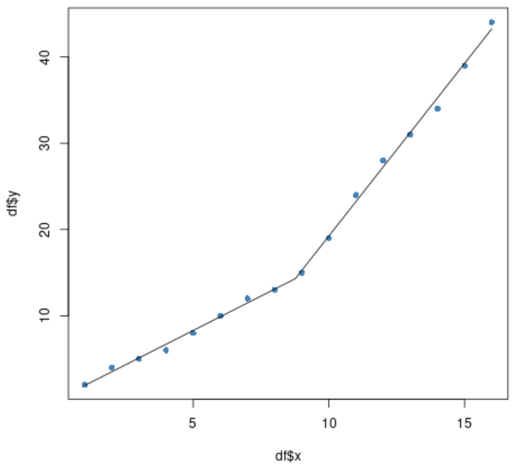
We can use the following code to visualize the final piecewise regression model on top of our original data:

#plot original data
plot(df$x, df$y, pch=16, col='steelblue')

#add segmented regression model
plot(segmented.fit, add=T)

It appears that the piecewise regression model fits the data quite well.

Additional Resources

The following tutorials provide additional information about regression models in R:

How to Perform Simple Linear Regression in R
How to Perform Multiple Linear Regression in R
How to Perform Logistic Regression in R
How to Perform Quantile Regression in R
How to Perform Weighted Regression in R