Often you may want to compare two columns in Google Sheets to look for similarities and differences.
The following examples show how to make the following comparisons between two columns:
1. Compare Two Columns to Find Which Values are Equal
2. Compare Two Columns to Find Which Values are Greater / Less Than
3. Compare Two Columns to Find Which Values Belong to Both Columns
Example 1: Find Which Values are Equal
We can use the following syntax to compare values across two columns and find which values are equal:
=IF(A1=B1, "Yes", "No")
The following screenshot shows how to use this syntax in practice:
This allows us to quickly see which values match in each row between the two columns.
Example 2: Find Which Values are Greater & Less Than
We can use the following syntax to compare values across two columns and find which values are greater:
=IF(A1>B1, "Team 1", "Team 2")
The following screenshot shows how to use this syntax in practice:
This allows us to quickly see which team scored more points in each row.
Example 3: Find Which Values Belong to Both Columns
Suppose we have the following two columns and we want to find which values in column B also belong to column A:
We can use Conditional formatting to accomplish this.
First, highlight cells B2:B13. Then click the Format tab and then click Conditional formatting:
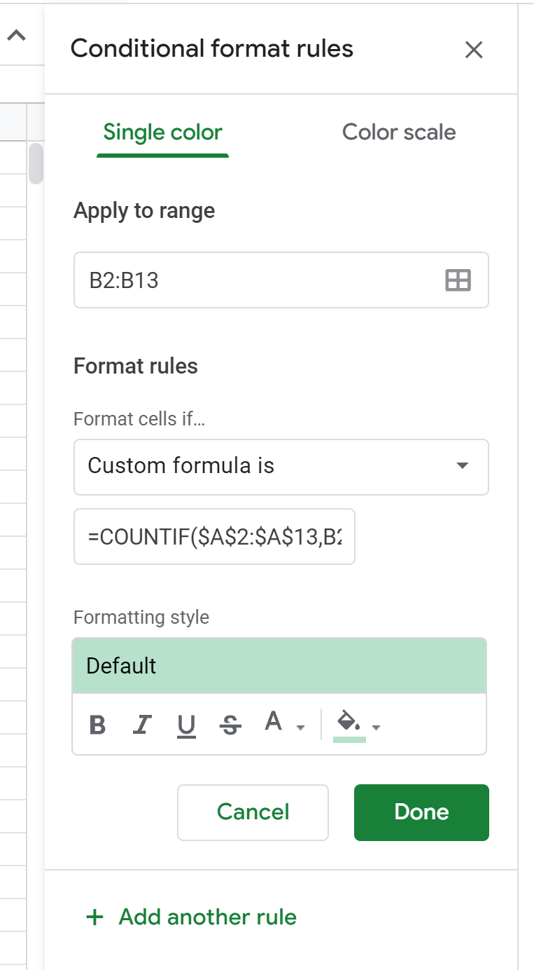
In the Conditional format rules panel that appears on the right side of the screen, click the dropdown menu next to Format cells if… and scroll to the bottom of the list and click Custom formula is.
Then enter the following formula:
=COUNTIF($A$2:$A$13,B2)>0
Once you click Done, the conditional formatting will be applied to column B:
Notice that each value in column B that also appears in column A is highlighted.
Note that you can also change the color used for highlighting in the Conditional format rules panel.
For example, we could change the highlighting color to orange:
Additional Resources
The following tutorials explain how to perform other common operations in Google Sheets:
How to Combine Columns in Google Sheets
How to Use SUMIF with Multiple Columns in Google Sheets
How to Use COUNTIF with Multiple Ranges in Google Sheets


