An Introduction to the Exponential Distribution

The exponential distribution is a probability distribution that is used to model the time we must wait until a certain event occurs.

This distribution can be used to answer questions like:

• How long does a shop owner need to wait until a customer enters his shop?
• How long will a laptop continue to work before it breaks down?
• How long will a car battery continue to work before it dies?
• How long do we need to wait until the next volcanic eruption in a certain region?

In each scenario, we’re interested in calculating how long we’ll have to wait until a certain event occurs. Thus, each scenario could be modeled using an exponential distribution.

Exponential Distribution: PDF & CDF

If a random variable X follows an exponential distribution, then the probability density function of X can be written as:

f(x; λ) = λe^-λx

where:

• λ: the rate parameter (calculated as λ = 1/μ)
• e: A constant roughly equal to 2.718

The cumulative distribution function of X can be written as:

F(x; λ) = 1 – e^-λx

In practice, the CDF is used most often to calculate probabilities related to the exponential distribution.

For example, suppose the mean number of minutes between eruptions for a certain geyser is 40 minutes. What is the probability that we’ll have to wait less than 50 minutes for an eruption?

To solve this, we need to first calculate the rate parameter:

• λ = 1/μ
• λ = 1/40
• λ = .025

We can plug in λ = .025 and x = 50 to the formula for the CDF:

• P(X ≤ x) = 1 – e^-λx
• P(X ≤ 50) = 1 – e^-.025(50)
• P(X ≤ 50) = 0.7135

The probability that we’ll have to wait less than 50 minutes for the next eruption is 0.7135.

Visualizing the Exponential Distribution

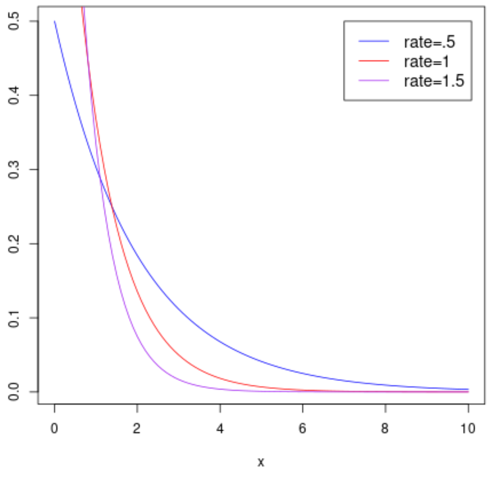
The following plot shows the probability density function of a random variable X that follows an exponential distribution with different rate parameters:

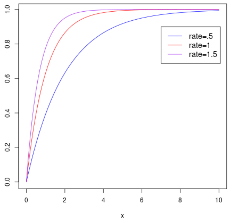
And the following plot shows the cumulative distribution function of a random variable X that follows an exponential distribution with different rate parameters:

Note: Check out this tutorial to learn how to plot an exponential distribution in R.

Properties of the Exponential Distribution

The exponential distribution has the following properties:

• Mean: 1 / λ
• Variance: 1 / λ²

For example, suppose the mean number of minutes between eruptions for a certain geyser is 40 minutes. We would calculate the rate as λ = 1/μ = 1/40 = .025.

We could then calculate the following properties for this distribution:

• Mean waiting time for next eruption: 1/λ = 1 /.025 = 40
• Variance in waiting times for next eruption: 1/λ² = 1 /.025² = 1600

Note: The exponential distribution also has a memoryless property, which means the probability of some future event occurring is not affected by the occurrence of  past events.

Exponential Distribution Practice Problems

Use the following practice problems to test your knowledge of the exponential distribution.

Question 1: A new customer enters a shop every two minutes, on average. After a customer arrives, find the probability that a new customer arrives in less than one minute.

Solution 1: The average time between customers is two minutes. Thus, the rate can be calculated as:

• λ = 1/μ
• λ = 1/2
• λ = 0.5

We can plug in λ = 0.5 and x = 1 to the formula for the CDF:

• P(X ≤ x) = 1 – e^-λx
• P(X ≤ 1) = 1 – e^-0.5(1)
• P(X ≤ 1) = 0.3935

The probability that we’ll have to wait less than one minute for the next customer to arrive is 0.3935.

Question 2: An earthquake occurs every 400 days in a certain region, on average. After an earthquake occurs, find the probability that it will take more than 500 days for the next earthquake to occur.

Solution 2: The average time between earthquakes is 400 days. Thus, the rate can be calculated as:

• λ = 1/μ
• λ = 1/400
• λ = 0.0025

We can plug in λ = 0.0025 and x = 500 to the formula for the CDF:

• P(X ≤ x) = 1 – e^-λx
• P(X ≤ 1) = 1 – e^-0.0025(500)
• P(X ≤ 1) = 0.7135

The probability that we’ll have to wait less than 500 days for the next earthquake is 0.7135. Thus, the probability that we’ll have to wait more than 500 days for the next earthquake is 1 – 0.7135 = 0.2865.

Question 3: A call center receives a new call every 10 minutes, on average. After a customer calls, find the probability that a new customer calls within 10 to 15 minutes.

Solution 3: The average time between calls is 10 minutes. Thus, the rate can be calculated as:

• λ = 1/μ
• λ = 1/10
• λ = 0.1

We can use the following formula to calculate the probability that a new customer calls within 10 to 15 minutes:

• P(10 -0.1(15))  –  (1 – e^-0.1(10))
• P(10
• P(10

The probability that a new customer calls within 10 to 15 minutes. is 0.1448.

Additional Resources

The following tutorials provide introductions to other common probability distributions.

An Introduction to the Normal Distribution
An Introduction to the Binomial Distribution
An Introduction to the Poisson Distribution
An Introduction to the Uniform Distribution