A Mann-Whitney U test (sometimes called the Wilcoxon rank-sum test) is used to compare the differences between two samples when the sample distributions are not normally distributed and the sample sizes are small (n
It is considered to be the nonparametric equivalent to the two sample t-test.
This tutorial explains how to perform a Mann-Whitney U test in Excel.
Example: Mann-Whitney U Test in Excel
Researchers want to know if a fuel treatment leads to a change in the average mpg of a car. To test this, they conduct an experiment in which they measure the mpg of 12 cars with the fuel treatment and 12 cars without it.
Because the sample sizes are small and they suspect that the sample distributions are not normally distributed, they decided to perform a Mann-Whitney U test to determine if there is a statistically significant difference in mpg between the two groups.
Perform the following steps to conduct a Mann-Whitney U test in Excel.
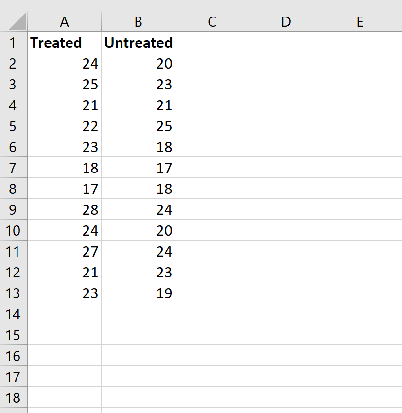
Step 1: Enter the data.
Enter the data as follows:
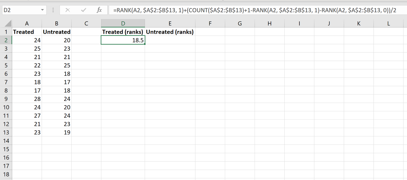
Step 2: Calculate the ranks for both groups.
Next, we’ll calculate the ranks for each group. The following image shows the formula to use to calculate the rank of the first value in the Treated group:
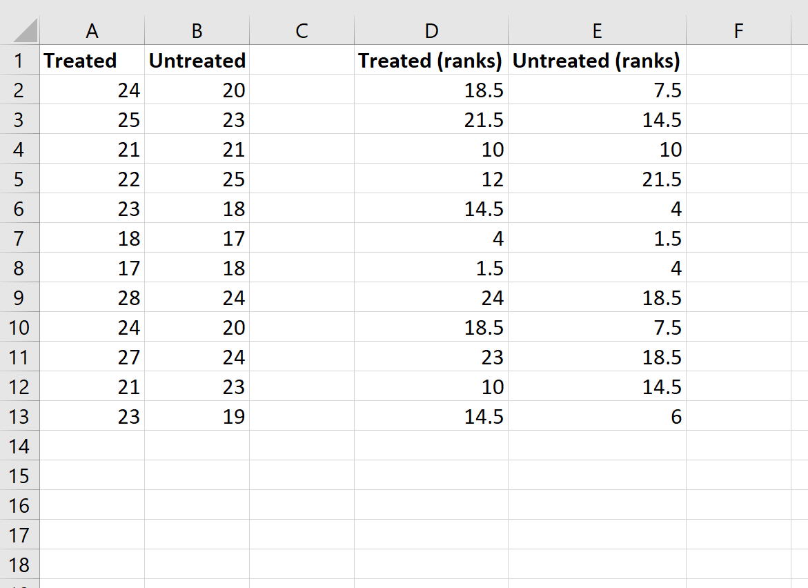
Although this formula is fairly complicated, you only have to enter it one time. Then, you can simply drag the formula to all of the other cells to fill in the ranks:
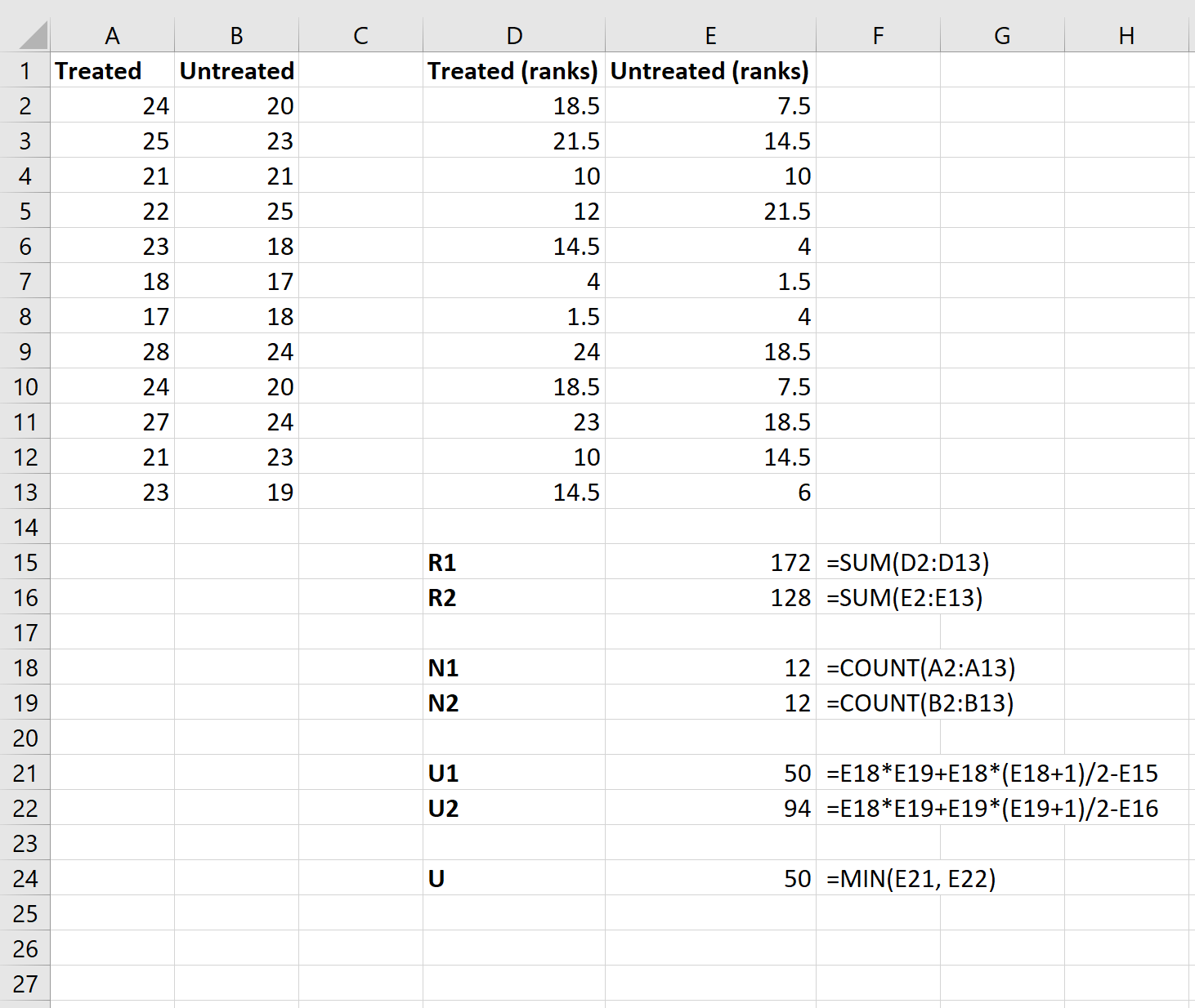
Step 3: Calculate the necessary values for the test statistic.
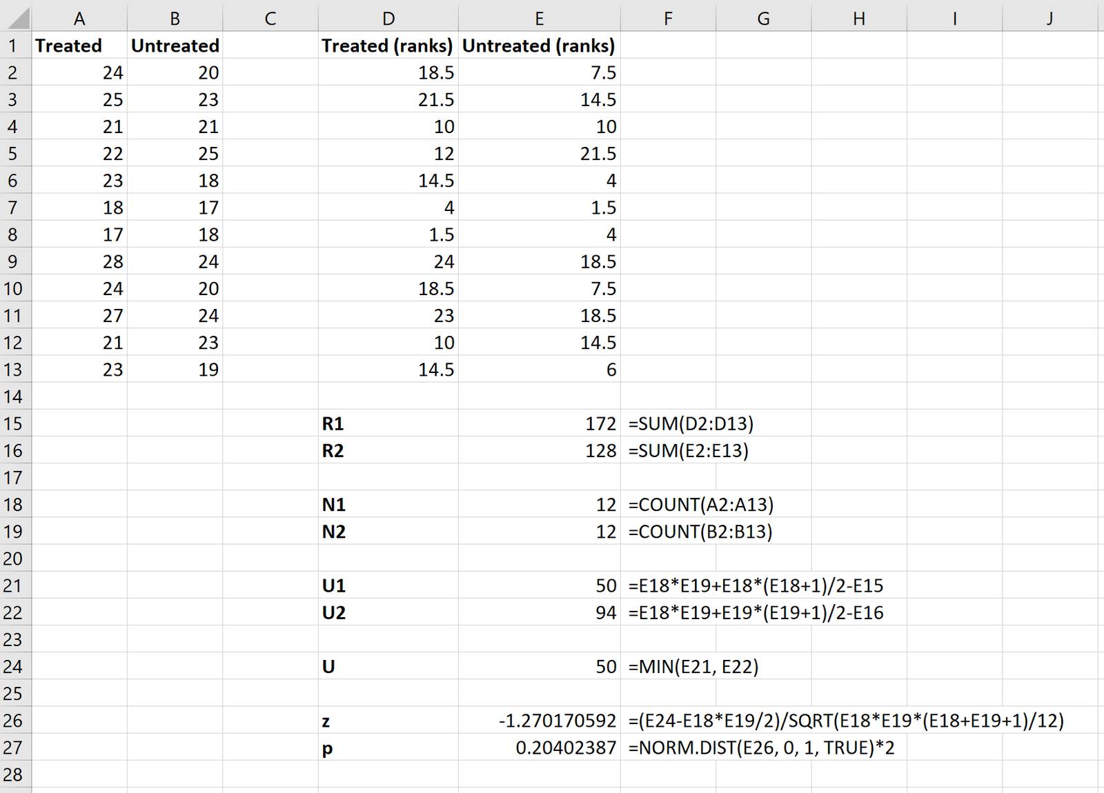
Next, we’ll use the following formulas to calculate the sum of the ranks for each group, the sample size for each group, the U test statistic for each group, and the overall U test statistic:
Step 4: Calculate the z test statistic and the corresponding p-value.
Lastly, we’ll use the following formulas to calculate the z test statistic and the corresponding p-value to determine if we should reject or fail to reject the null hypothesis:
The null hypothesis of the test states that the two groups have the same mean mpg. Since the p-value of the test is (0.20402387) is not smaller than our significance level of 0.05, we fail to reject the null hypothesis.
We do not have sufficient evidence to say that the true mean mpg is different between the two groups.


